Compute performance metrics from scratch

A Practical Guide to Computing Performance Metrics in Machine Learning from Scratch

Photo by Alexander Grey on Unsplash

Introduction:

Machine learning models are powerful tools that enable us to make accurate predictions and extract valuable insights from data. Evaluating the performance of these models is essential to understand their effectiveness and make informed decisions. While popular machine learning libraries provide pre-implemented performance metrics, understanding how to compute these metrics from scratch offers a deeper comprehension of their underlying principles and allows for customization to specific needs.

In this blog, we will embark on a journey to implement several key performance metrics from scratch. We will explore the computation of fundamental metrics such as the confusion matrix, f1-score, AUC score, accuracy score, MSE (Mean Squared Error), MAPE (Mean Absolute Percentage Error), and r2 score. By building these metrics step by step, we will gain a comprehensive understanding of their calculations, enabling us to evaluate machine learning models with precision and flexibility.

Whether you are a beginner looking to enhance your understanding of performance evaluation or an experienced practitioner seeking to gain a deeper insight into the metrics you use daily, this blog is for you. Throughout the process, we will emphasize the importance of these metrics in assessing model performance and provide practical code examples to illustrate their implementation.

Before we dive into the specifics of each metric, let’s briefly discuss the motivation behind computing performance metrics from scratch and the advantages it offers over relying solely on pre-implemented libraries. By building these metrics ourselves, we will not only comprehend the core principles behind them but also gain the ability to tailor them to unique scenarios or specialized models.

1. Confusion Matrix

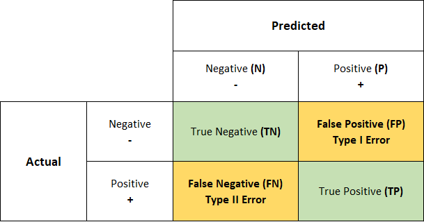
The confusion matrix is a fundamental performance metric in machine learning that provides a comprehensive overview of a classification model’s predictions. It offers valuable insights into the model’s accuracy by categorizing the predictions into true positives, true negatives, false positives, and false negatives. These categories represent the correct and incorrect predictions made by the model, allowing us to assess its performance in a more nuanced manner.

A confusion matrix presents a tabular representation of the model’s predictions against the actual labels of the dataset. The rows of the matrix correspond to the true labels, while the columns represent the predicted labels. Each cell in the matrix contains the count or frequency of instances falling into a particular category. For example, the top-left cell represents the number of true negatives, indicating the instances correctly classified as negative by the model.

The confusion matrix serves as the foundation for computing various evaluation metrics such as accuracy, precision, recall, and the f1-score. By analyzing the values within the matrix, we can understand the model’s strengths and weaknesses in correctly classifying different classes. This information is crucial for assessing the performance of our classification models, identifying potential biases or imbalances, and making informed decisions based on the model’s predictions.

https://miro.medium.com/v2/resize:fit:1218/1*jMs1RmSwnYgR9CsBw-z1dw.png

def get_confusion_matrix(y_true, y_pred):
    # Convert input arguments to arrays
    y_true = y_true.values
    y_pred = y_pred.values
    
    # Calculate True Negatives (TN)
    TN = ((y_true == 0) & (y_pred == 0)).sum()
    
    # Calculate True Positives (TP)
    TP = ((y_true == 1) & (y_pred == 1)).sum()
    
    # Calculate False Negatives (FN)
    FN = ((y_true == 1) & (y_pred == 0)).sum()
    
    # Calculate False Positives (FP)
    FP = ((y_true == 0) & (y_pred == 1)).sum()
    
    # Return the confusion matrix as a 2x2 numpy array
    return np.array([[TN, FP], [FN, TP]])

The get_confusion_matrix function takes two input arguments: y_true and y_pred. These arguments represent the true labels and predicted labels, respectively.

It’s important to note that this code assumes that y_true and y_pred are pandas Series objects, which is why the .values attribute is used to convert them to arrays.

Next, the confusion matrix values are calculated using a series of logical operations and sums. Here’s a breakdown of each line:

• TN = ((y_true == 0) & (y_pred == 0)).sum(): This line calculates the number of true negatives. It checks where both the true labels and predicted labels are equal to 0 (representing the negative class) and sums the occurrences.
• TP = ((y_true == 1) & (y_pred == 1)).sum(): Similarly, this line calculates the number of true positives. It checks where both the true labels and predicted labels are equal to 1 (representing the positive class) and sums the occurrences.
• FN = ((y_true == 1) & (y_pred == 0)).sum(): This line calculates the number of false negatives. It checks where the true labels are equal to 1 (positive class) and the predicted labels are equal to 0 (negative class), then sums the occurrences.
• FP = ((y_true == 0) & (y_pred == 1)).sum(): Likewise, this line calculates the number of false positives. It checks where the true labels are equal to 0 (negative class) and the predicted labels are equal to 1 (positive class), then sums the occurrences.

Finally, the function returns a 2x2 numpy array representing the confusion matrix. The array is structured as [[TN, FP], [FN, TP]], aligning with the layout of the confusion matrix: true negatives, false positives, false negatives, and true positives.

2. F1 Score

The f1-score is a widely used performance metric in machine learning that combines the concepts of precision and recall into a single measure. It provides a balanced evaluation of a classification model’s accuracy by considering both the ability to correctly identify positive instances (precision) and the ability to capture all positive instances (recall).

Precision represents the ratio of true positives to the total predicted positives, indicating the model’s accuracy in correctly classifying positive instances. On the other hand, recall, also known as sensitivity or true positive rate, measures the ratio of true positives to the total actual positives, reflecting the model’s ability to identify all positive instances.

The f1-score is the harmonic mean of precision and recall, providing a single value that takes into account both metrics. By considering both precision and recall, the f1-score offers a comprehensive assessment of a model’s performance, particularly when dealing with imbalanced datasets or scenarios where both high precision and recall are desired.

https://inside-machinelearning.com/wp-content/uploads/2021/09/F1-Score.png

def get_f1_score(y_true, y_pred):

    # get_confusion_matrix() is already implemented above

    TN, FP, FN, TP = get_confusion_matrix(y_true, y_pred).ravel()
    
    # Calculate precision score
    precision_score = TP / (TP + FP)
    
    # Calculate recall score
    recall_score = TP / (TP + FN)
    
    # Calculate f1-score
    f1_score = (2 * precision_score * recall_score) / (precision_score + recall_score)
    
    return f1_score

get_f1_score function takes two input arguments: y_true and y_pred. These arguments represent the true labels and predicted labels, respectively.

The first line of the function uses the get_confusion_matrix function (it has been previously defined above) to obtain the confusion matrix values: TN, FP, FN, and TP. The ravel() method is then applied to flatten the 2x2 matrix into a 1-dimensional array, allowing us to extract the individual values.

Next, the precision score is calculated by dividing the true positives (TP) by the sum of true positives and false positives (TP + FP). This represents the accuracy of positive predictions made by the model.

The recall score is calculated by dividing the true positives (TP) by the sum of true positives and false negatives (TP + FN). This measures the model’s ability to identify all positive instances.

Finally, the f1-score is computed by taking the harmonic mean of precision and recall. It is calculated as twice the product of precision and recall, divided by the sum of precision and recall. This provides a balanced measure of the model’s accuracy, considering both precision and recall.

Why is the f1-score the harmonic mean of precision and recall rather than the arithmetic mean?

3. AUC Score

The AUC (Area Under the Curve) score is a popular performance metric used in binary classification tasks, particularly in machine learning models that output probability scores. AUC represents the overall performance of a classifier by measuring the area under the Receiver Operating Characteristic (ROC) curve.

The ROC curve is a graphical representation that illustrates the trade-off between the true positive rate (TPR) and the false positive rate (FPR) at various classification thresholds. TPR is also known as recall or sensitivity, while FPR is defined as (1 — specificity).

To compute the AUC score, the ROC curve is created by calculating the TPR and FPR values at different classification thresholds. The curve is then used to determine the area under it. A perfect classifier would have an AUC score of 1, while a completely random classifier would have an AUC score of 0.5.

The AUC score provides a single value that represents the classifier’s ability to discriminate between positive and negative instances across all possible classification thresholds. It is robust to class imbalance and threshold selection, making it a valuable metric for evaluating the overall performance of binary classification models.

https://glassboxmedicine.files.wordpress.com/2019/02/roc-curve-v2.png

def get_auc_score(y_true, y_prob):
    # Create a DataFrame with true labels and predicted probabilities
    df = pd.concat([y_true, y_prob], axis=1)
    df.columns = ['y_true', 'y_prob']

    # Sort the DataFrame by predicted probabilities in descending order
    df.sort_values(by='y_prob', ascending=False, inplace=True)

    # Get an array of all possible threshold values
    threshold = df['y_prob'].values

    # Initialize empty arrays to store TPR and FPR values
    tpr_array = []
    fpr_array = []

    # Iterate over each threshold value
    for thres in threshold:
        # Predict labels based on the threshold
        y_pred = pd.Series(np.where(df['y_prob'] < thres, 0, 1))
        
        # Calculate the confusion matrix values
        TN, FP, FN, TP = get_confusion_matrix(df['y_true'], y_pred).ravel()

        # Calculate the true positive rate (TPR) and false positive rate (FPR)
        tpr = TP / (TP + FN)
        fpr = FP / (FP + TN)

        # Append the TPR and FPR values to the respective arrays
        tpr_array.append(tpr)
        fpr_array.append(fpr)

    # Calculate the AUC score by integrating the TPR and FPR values
    return np.trapz(tpr_array, fpr_array)

Calculates the AUC score by following these steps:

1. The function get_auc_score takes two input arguments: y_true, which represents the true labels, and y_prob, which represents the predicted probabilities of the positive class.
2. A new DataFrame named df is created by concatenating the y_true and y_prob arrays along the columns using pd.concat([y_true, y_prob], axis=1). The resulting DataFrame has two columns: 'y_true' and 'y_prob'.
3. The DataFrame is sorted in descending order based on the predicted probabilities (‘y_prob’) using df.sort_values(by='y_prob', ascending=False, inplace=True). This step ensures that the DataFrame is ordered correctly for calculating the ROC curve.
4. The array of predicted probabilities from the sorted DataFrame is obtained using threshold = df['y_prob'].values. Each value in threshold represents a different classification threshold that will be used to determine whether a prediction is classified as positive or negative.
5. Two empty arrays, tpr_array and fpr_array, are initialized. These arrays will store the true positive rate (TPR) and false positive rate (FPR) values at each threshold.
6. A loop is then executed for each threshold value in threshold. Inside the loop, the predicted labels (y_pred) are calculated based on the current threshold using pd.Series(np.where(df['y_prob'] < thres, 0, 1)). This assigns a value of 0 or 1 to each prediction, based on whether the predicted probability is below or above the threshold.
7. The confusion matrix values, TN, FP, FN, and TP, are obtained by calling the get_confusion_matrix function with the true labels (df['y_true']) and the predicted labels (y_pred). These values are then used to calculate the TPR and FPR.
8. The TPR and FPR values are appended to tpr_array and fpr_array, respectively, for each threshold.
9. Finally, the AUC score is computed using np.trapz(tpr_array, fpr_array), which calculates the area under the ROC curve based on the TPR and FPR values.

Alternate implementation of AUC score that is faster and more efficient:

def get_auc_score(y_true, y_prob):
    y_true = y_true.values
    y_prob = y_prob.values
    
    # Get indices that would sort y_prob in descending order
    sorted_indices = np.argsort(-y_prob)
    
    # Sort y_true using the same indices
    sorted_y_true = y_true[sorted_indices]
    
    # Compute total number of positive and negative samples
    num_positive = np.sum(sorted_y_true == 1)
    num_negative = np.sum(sorted_y_true == 0)
    
    # Initialize arrays for TPR and FPR
    tpr_array = []
    fpr_array = []
    
    cum_tp = np.cumsum(sorted_y_true == 1)
    cum_fp = np.cumsum(sorted_y_true != 1)
    
    tpr = cum_tp / num_positive
    fpr = cum_fp / num_negative

    tpr_array.append(tpr)
    fpr_array.append(fpr)
        
    return np.trapz(tpr_array, fpr_array)

This alternative implementation of the AUC score is faster and more efficient because it avoids sorting the entire DataFrame. Instead, it directly operates on the NumPy arrays (y_true and y_prob).

Here’s how the code works:

1. Convert y_true and y_prob to NumPy arrays using .values. This ensures that the code can handle both Pandas Series and NumPy arrays as inputs.
2. Use np.argsort(-y_prob) to obtain the indices that would sort the y_prob array in descending order. The - sign is used to sort in descending order.
3. Sort y_true using the sorted indices obtained in the previous step. This step ensures that y_true aligns with the sorted y_prob values.
4. Compute the total number of positive and negative samples by counting the occurrences of 1 and 0 in the sorted y_true array, respectively.
5. Initialize empty arrays for TPR and FPR.
6. Use np.cumsum(sorted_y_true == 1) and np.cumsum(sorted_y_true != 1) to calculate the cumulative sum of True Positives (cumulative sum of 1 in sorted_y_true) and False Positives (cumulative sum of values that are not 1 in sorted_y_true), respectively.
7. Calculate the TPR and FPR by dividing the cumulative True Positives and False Positives by the total number of positive and negative samples, respectively.
8. Append the TPR and FPR values to their respective arrays.
9. Finally, calculate the AUC score using np.trapz(tpr_array, fpr_array).

By using this alternative implementation, you can compute the AUC score efficiently and achieve faster results, especially for large datasets.

4. Accuracy Score

The accuracy score is a widely used performance metric in machine learning that measures the proportion of correct predictions made by a model over the total number of predictions. It provides an overall assessment of how well the model is able to classify instances correctly.

The accuracy score is calculated by dividing the number of correctly predicted instances (true positives and true negatives) by the total number of instances in the dataset. It is expressed as a value between 0 and 1, with 1 indicating perfect accuracy.

While accuracy is a useful metric, it may not be the best choice in scenarios where the classes are imbalanced or when different misclassification costs are involved. Therefore, it is important to consider the specific characteristics and requirements of the problem at hand when interpreting and evaluating the accuracy score.

https://www.nomidl.com/wp-content/uploads/2022/02/image-13.png

In this code, the get_accuracy_score_ function takes two arguments: y_true (true labels) and y_pred (predicted labels). It calculates the accuracy score based on these inputs.

First, the function calls the get_confusion_matrix function to obtain the confusion matrix values: true negatives (TN), false positives (FP), false negatives (FN), and true positives (TP). These values are then unpacked into the respective variables.

Next, the accuracy score is calculated by summing the number of true negatives and true positives and dividing it by the sum of all four values in the confusion matrix (TN + TP + FN + FP). The accuracy score represents the proportion of correctly classified instances over the total number of instances.

Finally, the calculated accuracy score is returned by the function.

An alternative implementation of the accuracy score without using the confusion matrix:

def get_accuracy_score(y_true, y_pred):
    # Calculate the total number of samples
    total_samples = len(y_true)
    
    # Count the number of correct predictions by comparing y_true and y_pred
    correct_predictions = sum(y_true == y_pred)
    
    # Calculate the accuracy by dividing the number of correct predictions by the total number of samples
    accuracy = correct_predictions / total_samples
    
    # Return the accuracy score
    return accuracy

The total_samples variable is assigned the length of y_true, representing the total number of instances in the dataset.

The correct_predictions variable is calculated using the sum function. It compares the elements of y_true and y_pred using the == operator, resulting in a boolean array. The sum function then sums the number of True values, representing the correct predictions.

The accuracy is calculated by dividing the correct_predictions by the total_samples, giving the proportion of correctly classified instances.

Finally, the accuracy score is returned by the function.

Compute performance metrics(for regression)

1. Mean Square Error

Mean Square Error (MSE) is a commonly used metric for evaluating the performance of regression models. It measures the average squared difference between the predicted and true values of the target variable. The MSE provides a measure of how close the predicted values are to the actual values, with lower values indicating better model performance.

To calculate the MSE, the squared differences between each predicted and true value are summed, and then divided by the total number of samples. The resulting value represents the average squared difference between the predicted and true values. The MSE is particularly useful when the errors in prediction need to be emphasized, as the squared differences amplify larger errors. However, it is sensitive to outliers in the data, as they can greatly affect the MSE value. Therefore, it is important to interpret the MSE in the context of the specific problem and consider other evaluation metrics as well.

https://cdn-media-1.freecodecamp.org/images/hmZydSW9YegiMVPWq2JBpOpai3CejzQpGkNG

def get_mse(y_true, y_pred):
    # Calculate the squared differences between y_true and y_pred
    squared_diff = (y_true - y_pred) ** 2
    
    # Calculate the mean of the squared differences
    mse = squared_diff.mean()
    
    # Return the mean squared error
    return mse

In this code, the get_mse function takes two arguments: y_true (true values) and y_pred (predicted values). It calculates the Mean Square Error (MSE) based on these inputs.

To compute the MSE, the implementation uses the mathematical formula: the squared differences between each corresponding pair of y_true and y_pred. This is achieved by subtracting y_pred from y_true and then squaring the result using the expression (y_true - y_pred) ** 2. This step ensures that all differences are positive and emphasizes larger errors due to the squaring operation.

Next, the .mean() function is applied to the squared differences. It calculates the average of all the squared differences, resulting in the MSE value.

2. Mean Absolute Percentage Error

Mean Absolute Percentage Error (MAPE) is a metric commonly used to measure the accuracy of a forecasting or prediction model, particularly in time series analysis. It calculates the average percentage difference between the predicted and true values of the target variable. MAPE is expressed as a percentage, providing a relative measure of the magnitude of errors.

To calculate the MAPE, the absolute differences between each predicted and true value are divided by the true values, and then averaged across all samples. This normalization by the true values allows for comparison across different scales and magnitudes of the target variable.

MAPE provides insights into the relative accuracy of the model’s predictions. A lower MAPE indicates better model performance, as it signifies smaller average percentage differences between predictions and ground truth. However, it is important to note that MAPE has limitations, such as being sensitive to zero or near-zero true values and infinite values for perfect predictions. Therefore, it is crucial to interpret the MAPE alongside other evaluation metrics and consider the specific characteristics of the problem at hand.

def get_mape(y_true, y_pred):
    return np.mean(np.abs((y_true - y_pred) / y_true))

In this code, the get_mape function takes two arguments: y_true (true values) and y_pred (predicted values). It calculates the Mean Absolute Percentage Error (MAPE) based on these inputs.

To compute the MAPE, the implementation first calculates the absolute differences between each corresponding pair of y_true and y_pred using the expression np.abs((y_true - y_pred)). This step ensures that all differences are positive, regardless of the direction of the error.

Next, the absolute differences are divided by the true values y_true using the expression ((y_true - y_pred) / y_true). This division normalizes the differences by the true values, allowing for comparison across different scales and magnitudes of the target variable. The result is an array of relative errors, representing the percentage difference between the predicted and true values.

Finally, the np.mean function is applied to the array of relative errors. It calculates the average of all the relative errors, resulting in the MAPE value.

When using this implementation, it is important to note that MAPE may not be appropriate in all scenarios. For example, it can encounter issues when the true values are close to zero or when perfect predictions result in infinite MAPE values. Therefore, it is recommended to interpret the MAPE alongside other evaluation metrics and consider the specific characteristics and requirements of your problem.

So instead of using the above implementation where we are dividing the error with true values, now we divide with mean value of true value

def get_mape(y_true,y_pred):
    y_true_mean = y_true.mean()
    return np.mean(np.abs((y_true-y_pred)/np.abs(y_true_mean)))

In this code, the get_mape_1 function takes two arguments: y_true (true values) and y_pred (predicted values). It calculates the Mean Absolute Percentage Error (MAPE) based on these inputs.

To compute the MAPE, the implementation first calculates the mean of the true values using y_true.mean() and assigns it to y_true_mean. This value represents the average of the true values and is used as the denominator for normalization.

Next, the implementation calculates the absolute differences between each corresponding pair of y_true and y_pred using np.abs((y_true - y_pred)). This ensures that all differences are positive, regardless of the direction of the error.

Then, the implementation divides the absolute differences by the absolute value of y_true_mean using (y_true - y_pred) / np.abs(y_true_mean). This division normalizes the differences by the average magnitude of the true values, allowing for comparison across different scales and magnitudes of the target variable.

Finally, the np.mean function is applied to the array of relative errors. It calculates the average of all the relative errors, resulting in the MAPE value.

It’s important to note that there are different variations and interpretations of MAPE, and different implementations may exist depending on the specific context and requirements of your problem. When using MAPE, it’s advisable to consider its limitations and interpret the results in conjunction with other evaluation metrics to gain a comprehensive understanding of model performance.

3. R-squared (R²) error

The R-squared (R²) error, also known as the coefficient of determination, is a metric used to evaluate the performance of a regression model. It measures the proportion of the variance in the dependent variable that can be explained by the independent variables in the model.

R² error ranges from 0 to 1, where 0 indicates that the model does not explain any of the variability in the dependent variable, and 1 indicates that the model perfectly explains all the variability. In some cases, R² can also be negative, which suggests that the model performs worse than a simple horizontal line.

To calculate R² error, we compare the sum of squares of the residuals (SSR) to the total sum of squares (SST). The residual is the difference between the predicted and actual values for each data point. SST measures the total variability of the dependent variable.

A higher R² value indicates a better fit of the regression model to the data. However, it’s important to note that R² should not be the sole criterion for model evaluation. It is possible to have a high R² value even if the model is overfitting or if it has omitted relevant independent variables.

def get_r2_square(y_true, y_pred):
    # Calculate the mean of the true values
    y_true_mean = y_true.mean()
    
    # Calculate the sum of squares of the residuals (SSres)
    SSres = ((y_true - y_pred) ** 2).sum()
    
    # Calculate the total sum of squares (SStot)
    SStot = ((y_true - y_true_mean) ** 2).sum()
    
    # Calculate the R^2 square using the formula
    r2_square = 1 - (SSres / SStot)
    
    # Return the R^2 square
    return r2_square

1. Calculate the mean of the true values:

• y_true_mean = y_true.mean()
• This line calculates the average of the true values y_true using the mean() function.

2. Calculate the sum of squares of the residuals (SSres):

• SSres = ((y_true - y_pred) ** 2).sum()
• This line calculates the sum of the squared differences between the true values y_true and the predicted values y_pred.
• It subtracts y_pred from y_true, squares the differences, and then sums them up using the sum() function.

3. Calculate the total sum of squares (SStot):

• SStot = ((y_true - y_true_mean) ** 2).sum()
• This line calculates the sum of the squared differences between the true values y_true and their mean value y_true_mean.
• It subtracts y_true_mean from y_true, squares the differences, and then sums them up using the sum() function.

4. Calculate the R² square:

• r2_square = 1 - (SSres / SStot)
• This line computes the R² square using the formula: 1 — (SSres / SStot).
• It divides SSres by SStot, subtracts the result from 1, and assigns the value to r2_square.

5. Return the R² square:

• return r2_square
• This line returns the computed R² square value as the output of the function.

In conclusion, we have explored the implementation of various performance metrics from scratch in the context of machine learning. By understanding the mathematical foundations and logic behind these metrics, we have gained insights into how they assess the quality and accuracy of our models.

Starting with the confusion matrix, we delved into its components, such as true positives, true negatives, false positives, and false negatives, which provide valuable information about classification results. We then moved on to metrics like F1-score and AUC score, which consider precision, recall, and the trade-off between true positives and false positives.

Accuracy score provided a straightforward measure of overall accuracy, while mean squared error (MSE) quantified the average squared difference between predicted and true values, assessing the performance of regression models. Mean absolute percentage error (MAPE) gave us a measure of the average percentage deviation from the true values, which is particularly useful when dealing with relative errors.

Lastly, we explored the R-squared (R²) score, a popular metric for regression models, which indicates the proportion of the variance in the dependent variable that is predictable from the independent variables.

By implementing these metrics from scratch, we have gained a deeper understanding of their inner workings and how they contribute to evaluating the performance of machine learning models. Armed with this knowledge, we can make more informed decisions in model selection, optimization, and performance evaluation.

Remember that these implementations provide a solid foundation for understanding performance metrics. However, in practical scenarios, it is often more efficient and convenient to use existing libraries and frameworks that offer pre-implemented functions for these metrics. These libraries not only save time but also ensure accurate and optimized calculations.

As you continue your journey in machine learning, I encourage you to explore these metrics further, experiment with different models and datasets, and continually refine your understanding of performance evaluation. With a solid grasp of these concepts, you’ll be better equipped to assess and improve the effectiveness of your machine learning models.

Happy coding and may your machine learning endeavors be successful!❤