Speech Command Classification using PyTorch and torchaudio
When I first started working on audio data I was scared a lot. Compared to image data, audio data seemed to me like an alien language. I still don’t claim to understand all the things but I can say a little bit about it so that the newcomers in this field feel more comfortable with it. I have used PyTorch and TorchAudio here to implement this project. Btw, if you need to brush up your basic signal processing skills you can look in to these videos here. It also contains a lot of tutorials for implementations as well.
Download Dataset
For this tutorial we will be classifying speech commands. It is a multi-class classification problem. There are a total of 105830 audio files of 35 classes each of them sampled at 16KHz. You can find this dataset and more from the torchaudio library. You can download it using the following code section.
dataset = torchaudio.datasets.SPEECHCOMMANDS('./data1/' , url = 'speech_commands_v0.02', folder_in_archive= 'SpeechCommands', download = True)Each item here is a tuple in the form of waveform, sample_rate, label, speaker_id, utterance_number. We will be using the waveform and label for training our model and use the sample_rate for understanding the data more clearly.
Visualization & Pre-processing
Let’s take the first tuple from the dataset and print their values and visualize them.
(tensor([[-0.0004, -0.0003, -0.0003,  ..., -0.0019, -0.0018,  0.0060]]),
 16000,
 'nine',
 'af790082',
 1)
So, we get a tensor of the raw audio file, it’s sampling rate of 16khz, it’s label, speaker_id and utterance_number. The shape of the raw audio file is 1x16000 implying that the audio file is of 1 second in length. Let’s visualize the raw waveform now then.
plt.figure()
plt.plot(dataset[0][0].t())
plt.show()
We can also easily load a single audio file using torchaudio.load() method. It returns the waveform and its sampling rate.
filename = "./SpeechCommands/speech_commands_v0.02/backward/0165e0e8_nohash_0.wav"
waveform, sample_rate = torchaudio.load(filename)plt.figure()
plt.plot(waveform.t().numpy())

After inspecting the waveform and the label we can understand two things. First, the labels are in text so we need to convert them into class numbers. Second, we need to verify that all the data samples are of equal length i.e. 1x16000. Both of them can be done easily. My approach may not be the easiest or the fastest but it is a simple approach.
For, the first problem I just created a list of the class labels using os.listdir() on the dataset folder where it was stored. Now, while loading the data we can use the class label lists index number to assign a number to the text labels.
import osaudio_path = './data1/SpeechCommands/speech_commands_v0.02/'labels_dict = os.listdir(audio_path)
###we can use the index() method to get the index number of an ###element. Here, labels are the text labels. idx represent any ###integer between 0 to 95393out_labels = label_dict.index(labels[idx])
To tackle with the second problem I just dropped the waveforms which weren’t equal to shape of 1x16000. After dropping we get 95394 data samples. We lost only approximately 10,000 samples. There are other ways we can do this but for initial stage this is enough. Since, we are interested in only the waveforms and their labels we only store these.
wave = []
labels = []
for i in range(0,105829):
    if dataset[i][0].shape == (1,16000):
        wave.append(dataset[i][0])
        labels.append(dataset[i][2])
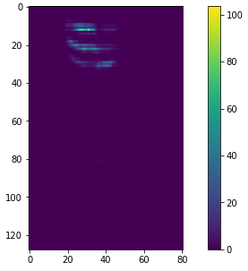
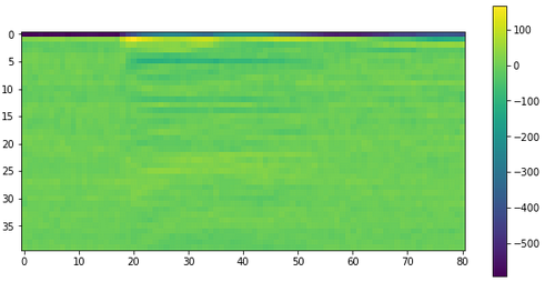
Now, that we have our waveforms and labels in order we need to think about in which approach we are going to process our data. We can use the raw waveform as it as for our deep neural network model to perform classification task. Otherwise, we can use features from the waveform. Popular features for audio processing include Mel-Spectogram which is a composition of Spectrogram and MelScale. We can also go for the MFCC features as well. Luckily we can get all these three transformations and many more using torchaudio library. In this tutorial I will be using all three of them separately and train three different models. (MelSpectogram and MFCC are like images so the DNN model has to be changed accordingly). Let’s visualize the MelSpectogram and MFCC representation.
###change MFCC to MelSpectogram to get Mel-scale Spectogramspecgram = torchaudio.transforms.MFCC()(wave[0])plt.figure(figsize=(10,5))
plt.imshow(specgram[0,:,:].numpy())
plt.colorbar()
plt.show()


Data Loader
Generally, the DataLoaders are used to load data in batches during runtime. For this reason in most cases file names and file directories are passed on to the class. Here, I didn’t do that instead I passed the list of waveforms and labels to the class. It returned in batches, the transformed waveform and labels in integers. You can have a look at the class that I created here.
class SpeechDataLoader(Dataset):

    def __init__(self,data,labels,list_dir,transform=None):
        self.data = data
        self.labels = labels
        self.label_dict = list_dir
        self.transform = transform

    def __len__(self):
        return len(self.data)

    def __getitem__(self,idx):
        waveform = self.data[idx]

        if self.transform != None:
            waveform = self.transform(waveform)        if self.labels[idx] in self.label_dict:
            out_labels = self.label_dict.index(self.labels[idx])        return waveform, out_labels
This will return transformed waveforms and labels in batches when called. If no transformation is passed on then it will use original raw waveform.
As we can see we need to split our dataset to get the training set, validation set and testing set. Here, I used torch.utils.data.random_split. It shuffles all the data and splits the data into training set and testing set.
from torch.utils.data import DataLoader,random_split,Datasetdataset= SpeechDataLoader(wave,labels,labels_dict)traindata, testdata = random_split(dataset, [round(len(dataset)*.8), round(len(dataset)*.2)])trainloader = torch.utils.data.DataLoader(traindata, batch_size=100, shuffle=True)testloader = torch.utils.data.DataLoader(testdata, batch_size=100, shuffle=True)
Model Training & Results
In this tutorial, I trained three separate models. One on raw waveform, one on MFCC and the last one on MelSpectogram. Since, the last two ones are like images I need to used conv2d and for the first one I need to use conv1d. The model summary for different input shapes are given here. The implementation of these models can be found in my repository.


For the optimizer, I used AdamW and I used Cyclic Learning Rate scheduler. I performed this experiment for all the models for 50 epochs.
After training the models, I achieved 82.21% accuracy for raw wavform, 74.34% accuracy for the MFCC and for the MelSpectogram, 84.23% accuracy.
In order to improve the results one can try to tweak the hyper-parameters of the model. One can also change the model and see what happens. Full implementation can be found in my github repository.