A practical approach to handle imbalanced class problems.
This article provides information about what is imbalanced class, methods to overcome imbalanced class problems, how one can evaluate it, cost sensitive learning, with practical demonstration.
Hey folks! today I am going to cover a very interesting yet very important topic of Machine Learning, let’s dive right into it.
What is Imbalanced class?
Suppose you have two classes where one class is positive and another is negative. Now in order to make good predictions your model needs to have a balanced data ratio for both these classes, a slight variation in ratio might not affect the prediction(e.g. 6:4) but if you have a large amount of data for one class and very small amount for other class(e.g. 1:100) then this creates poor or biased model performance. In the figure 1 below we can see the blue fish class has a very large amount of data and for the red fish class there isn’t sufficient data.
Problems like fraud detection, anomaly detection, spam detection, outlier detection can inherently have class imbalance.

Different ways used to tackle class imbalance:
Here we need to know the terms Majority and Minority class.
Let’s take an example of cancer patients where we have more data for the non cancer patients and less data for the actual cancer patients.
Majority class: The class which contains the larger part of the dataset, this class often contains negative or normal cases in dataset.
Minority class: The class which contains very few parts of the dataset, this class often possesses positive or abnormal cases in dataset.
1) Resampling Methods:
Method 1:
Under sampling: It is performed on the majority class by excluding samples of this class to get the balanced class distribution. The drawback of using this method is some of the samples which might be very helpful in model prediction are excluded.
Method 2:
Over sampling: It is performed on the minority class by duplicating the available samples, but just duplicating examples can not add any new information to the dataset. Instead we can use SMOTE (Synthetic Minority Oversampling Technique). The figure 2 demonstrates SMOTE well, as we can see the orange squares are minority class to make them approximately equal to majority class synthetic samples are generated by creating samples between the existing sample and its neighbouring samples (green squares) to achieve the balanced class distribution.

Method 3:
Combined Over & Under sampling: For getting more profound results we can combine both under and over sampling together. The combined methods are as follows.
1) SMOTE + Edited nearest neighbour
2) SMOTE + Tomek links
For using these methods you will need to install Python’s Imbalance learn library .
2) Using ensemble techniques:
There are some algorithms which gives better performance even if the data is imbalanced they are called ensemble methods. Ensemble methods works with the basic principle of combining many weak learner and create a strong learner which will improve the prediction results. There are two types of ensemble methods bagging and boosting.
A)Bagging or Bootstrap Aggregating :
In this technique many weak classifiers are combined in parallel manner, training the algorithms on each bootstrapped algorithm separately to give aggregation of the prediction at the end.
Bagging reduces overfitting, improves the accuracy of the predictions.

Above figure explains the bagging technique, here random samples of the training dataset are created and passed through different classifiers. Each classifier produces its own prediction, the final prediction is the aggregation of all the predictions.
B)Boosting:
In this technique, each model is trained sequentially, trying to correct its predecessor. For every iteration classifiers places more weights to those cases which where incorrectly classified in the last round, illustrated in figure below.

Types of boosting:
1)Adaptive boosting (AdaBoost):
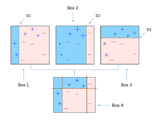
AdaBoost combines multiple weak learners to create a single strong learner. Initially all samples have same weights, after the first decision stump is given more weights are assigned to the observations which were incorrectly classified than the ones which classified correctly. In the figure below D1 is the first decision stump made to separate (+) and ( — ), but there are some (+) which are misclassified, these (+) will now have more weight and they will be fed to the second learner. The model will repeat these steps and adjust the errors until the most accurate model is built.

2)Gradient Boosting:
Gradient Boosting follows sequential model training. Both AdaBoost and Gradient Boosting work with weak learners to create a strong learner, but there is a major difference in these methods, unlike AdaBoost Gradient Boosting does not increase the weight of the misclassified objects instead it calculates residual error of the previous predictor and use it to fit the new predictor this is illustrated in the figure below.

3)XGBoost:
This is the more advanced version of gradient boosting and it stands for Extreme Gradient Boosting. Gradient boosting is very slow as it uses sequential model training hence they are not much scalable. XGBoost focuses on both computational speed and model performance. It uses parallel learning and is much faster than Gradient Boosting. In this users can define custom optimisation objective and evaluation criteria.
How to evaluate Imbalanced classification?
Choosing a right evaluation metrics is very important and challenging in machine learning but for imbalanced classification problem it is particularly difficult because most of standard metrics used assume to have a balanced class distribution.
Typically most widely used metric is accuracy, which is improper for imbalanced class problem as the high accuracy can be achieved even when model only predicts majority class. Here are few other evaluation metrics which can be used in case of imbalanced class problem.
Confusion Metrics: It is a table which shows values of correct and incorrect predictions, i.e values of True Positives, True Negatives, False Positives, False Negatives. Confusion metrics provides detailed insights for correct or incorrect class predictions along with the type of errors made during this classification i.e. false negative or false positive errors.
Sensitivity or Recall: It provides true positive rates, It is the ratio of correctly predicted positive examples by the total number of positive examples that could have been predicted. The number of false negatives reduces as the recall value increases.
Sensitivity or Recall = True Positives / (True Positives + False Negatives)
Specificity: It provides true negative rate i.e how well the negative class was predicted.
Specificity = TrueNegative / ( TrueNegative + FalsePositive )
Geometric mean or G-Mean: A single score for sensitivity and specificity is given by G-mean.
G-Mean = sqrt(Sensitivity * Specificity)
Precision: It is the ratio of correctly predicted positive examples by total correct examples that were predicted positive . The number of false positives reduces as the precision increases.
Precision = True Positives / (True Positives + False Positives)
F-Score or F-measure: It provides the overall model performance, F-score considers both precision and recall values.
F-Score = 2 * Precision * Recall / (Precision +Recall)
Matthews correlation coefficient: The MCC is a correlation coefficient between predicted and observed class and it varies from -1 to 1, where -1 shows disagreement in observed and predicted class, 1 shows perfect prediction and 0 shows no better than a random prediction.
MCC = (TP * TN)- (FP * FN) / sqrt ((TP+FP)(TP+FN)(TN+FP)(TN+FN))
Cost-sensitive learning:
Machine learning algorithms assumes that all the misclassification errors are equal, but for imbalanced classification problems classifying an ill patient as healthy(false negative) is more dangerous than classifying a healthy patient as ill(false positive).Cost sensitive learning takes these cost of the prediction errors into account and assigns a penalty for misclassification errors for each class.
Here in this tutorial we will be using logistic regression, the logistic regression uses sigmoid activation which maps the output value between 0 and 1. It is defined as 1 / (1+e^(-z)) which is shown in figure below.

The Cross-Entropy loss or the log loss is divided into two separate cost functions one for y=1 and one for y=0 as follows

which can be further compressed as

Hence the cost function of the model will be summation of all the training samples as shown below.

The scikit-learn library provides the class_weight attribute for a range of algorithms. The weights are inversely proportional, for example if we have a dataset with 0.99 and 0.01 class distribution for majority and minority class respectively then the penalty of 0.01 is assigned for the error of misclassifying majority class and 0.99 is assigned for the error of misclassifying minority class. This can be configured automatically by setting class_weight argument to “balanced”.
Let’s take an example of resampling method for imbalanced classification. Here we will create synthetic data and use logistic regression for model training. For step 1 import the necessary libraries for this example, then using make_classification a scikit_learn function, create a dataset of 10,000 samples which has class distribution of of [0.99] which means 99% of the data will belong to the majority class.
Next we will create a function to visualise our data, perform the train test split, train the logistic regression model, predict the output and observe the evaluation metrics.
We will first train our model without applying any sampling methods and observe the results.

In the above code we have more false negatives, recall and F-score are very less which makes the accuracy parameter dangerously misleading here. Now we will try the above mentioned sampling methods one by one and will make argument class_weight=”balanced” for further processing.

After performing under sampling the recall and F-score are increased more from the previous step but here the disadvantage of using only under sampling is that, data samples that might be helpful for model prediction has been deleted. Now let’s try over sampling using SMOTE.

In this case false negatives are less than false positives hence Recall and F-score has increased but we still have large number of false negatives and false positives, let’s combine over and under sampling methods and observe the results.

Using SMOTE +ENN has drastically reduced false negatives. There are more false positive cases than false negatives but the cost associated with them is less. Now the model has good recall, precision and F-score, so we can consider the accuracy as legitimate.
Imbalanced class handling in Deep Learning can be achieved by doing the weight balancing by assigning more weight to the misclassification of minority data or we can use the Focal Loss. Resampling methods like under and over sampling can be applied here too. We will see more about this in the next article.
Try the code by yourself, run the code, tweak the code and explore more!!!
Bye bye !!!!!!
https://machinelearningmastery.com/cost-sensitive-learning-for-imbalanced-classification/
