Evolution of Recommendation Algorithms, Part I: Fundamentals , History Overview, Core and Classical Algorithms

41 min readMar 25, 2024

A Comprehensive overview of Recommendation Algorithms and Evolution

Soon after the invention of the World Wide Web, the recommender
system emerged and related technologies have been extensively
studied and applied by both academia and industry. Currently, recommender system has become one of the most successful web
applications, serving billions of people in each day through recommending different kinds of contents, including news feeds, videos, e-commerce products, music, movies, books, games, friends, jobs etc. These successful stories have proved that recommender system can transfer big data to high values. This article briefly reviews the history of recommender systems, mainly from recommendation models view.

In this series we will have a extensive review to evolution of recommendation algorithms to know the dots about the progress of recommender systems, and the dots will somehow connect in the future, which inspires us to build more advanced recommendation services for changing the world better.

This series include five parts:

Part I: Fundamentals , History Overview and Classical Algorithms
Part II: Deep Recommendation Algorithms (TBD)
Part III: Hybrid Recommendation Algorithms (TBD)
Part IV: Advanced Recommendation Algorithms (TBD)
Part V: LLM Based Recommendation Algorithms (TBD)

I will cover basic concept, fundamentals and techniques in context of each article domain. We will use open source python packages for code and illustration of algorithms and techniques such as surprise,xLearn, implicit, LensKit, LighghFM, Recommenders , LibFFM and pytorchFM as well as some LLM based libraries like P5 recommender.

Business Perspective

Recommendation systems influence the way we shop online, stream movies, listen to music, and many other activities like find job. They analyze data about users, as well as any items/ services in question, to make predictions about what a user is most likely to be interested in. Consequently, these systems suggest products, services, items, etc., based on users’ preferences and previous actions, in combination with the items’ characteristics.

Netflix and IMDB use a recommendation engine to suggest movies you might like to watch, and Amazon uses one to offer you products you’re likely to buy. By providing users with recommendations that match their needs or desires, recommendation engines can increase conversion rates and unlock extra revenue at checkout, while giving customers a more personalized experience. That’s why well-designed recommendation engines are highly desirable for online commerce businesses.

More complicated, LinkedIn’s recommendation engine analyzes a user’s profile, work experience, skills, and job preferences to suggest relevant job opportunities. It takes into account factors such as location, industry, and job function to provide personalized job recommendations aligned with a user’s career interests.

Recommendation systems help businesses in increasing their conversion rate KPIs and unlocking extra revenue. Recommendation engines can also improve customer retention if customers are given suggestions that align well with their personal preferences, increasing their brand loyalty in the process.

**Fig 1. Recommendation Systems applications (Image by author)**

An amazing application of recommendation system is eco-friendly routing in google maps. With this capability you can choose a route that’s optimized for lower fuel consumption, which helps you save money on fuel and reduce carbon emissions something that’s top of mind for many Europeans. And this is a real concern — according to Statista’s 2022 report, road transportation is the largest source of carbon emissions throughout Europe. Although recommendation systems heavily rely on user preferences, while eco-friendly routing prioritizes environmental impact over user preferences (unless the user chooses to enable it).But that’s an interesting scenario! If users can enable a preference for eco-friendly routing, then it starts to blur the line between a traditional recommendation system and its current implementation in Google Maps. With user preference enabled, the system personalizes the routing based on a user’s stated eco-conscious preference. This aligns with a core aspect of recommender systems — tailoring suggestions based on user desires. Arguments for considering it a recommendation system is that the system presents an alternative route (eco-friendly) compared to the potentially faster or more familiar default route. This echoes how recommender systems suggest items or actions outside a user’s typical choices.

On the flip side of the coin, the most significant benefit of recommendation systems for customers is enabling them to consume or purchase more personalized content or items that are tailored to their own likings. This, in turn, leads to a more satisfying and engaging experience. Additionally, recommendation systems can help users in finding new content that they might like but find it too difficult to find otherwise. In other words, when developed carefully, recommendation systems can increase exposure to different perspectives.

**Fig 2.History of Amazon recommendation system evolution (Image by author)**

Basic Concepts

A recommendation system is a software tool or technique that automatically suggests relevant items (products, movies, music, job etc.) to users based on their preferences and past interactions. These systems play a crucial role in various online platforms, aiming to personalize the user experience by:

Improving user engagement: By suggesting items users are likely to enjoy, recommendation systems encourage them to spend more time and interact more actively with the platform.
Boosting conversions: By recommending relevant products, items, services, recommendation systems can increase the likelihood of users purchasing or taking desired actions within the platform.
Enhancing user satisfaction: By providing relevant suggestions, recommendation systems can create a more enjoyable and personalized user experience, leading to increased satisfaction and loyalty.

[ — ] Components: Understanding Relationship

Relationships provide recommender systems with tremendous insight . There are three main types that occur:

User-Item Relationship

The user-item relationship occurs when some users have an affinity or preference towards specific items that they need. For example, a cricket player might have a preference for cricket-related items, thus the e-commerce website will build a user-product relation of player->cricket.

Item-Item Relationship

Item-Item relationships occur when items are similar in nature, either by appearance or description. Some examples include books or music of the same genre, dishes from the same cuisine, or news articles from a particular event.

User-User Relationship

User-user relationships occur when some customers have similar taste with respect to a particular product or service. Examples include mutual friends, similar backgrounds, similar age, etc.

[ — ] Data and Recommender Systems

In recommender systems, data plays a vital role in understanding user preferences and suggesting relevant items. Here’s the two main types of data used in these systems:

1. User Data:

Information about the users interacting with the system. It can be broadly categorized into two sub-types:

Explicit Feedback: This data explicitly reflects a user’s preferences or opinions about items. It can include:

Ratings: Users provide star ratings, thumbs up/down, or numerical scores indicating their liking or disliking for an item.
Wishlist/Favorites: Adding items to a wishlist or marking them as favorites indicates a user’s interest in those specific items.
Explicit Search Queries: Keywords or phrases used by users to search for items can reveal their interests and intent.
Reviews: written text expressing opinions about an item, recommender systems can analyze the sentiment expressed in reviews (positive, negative, or neutral) to infer user preferences.
Following/Subscribing: Users follow or subscribe to specific creators, brands, or categories, revealing their general preferences within the system.
Item Comparison: Systems might present users with two or more items and ask them to choose their preferred option, providing explicit feedback for comparison.
Preference Elicitation: Recommender systems might ask users direct questions about their preferences for specific features or attributes to gather explicit feedback.

Implicit Feedback: This data indirectly reflects a user’s preferences based on their interactions with the system. It can include:

Browsing History: The items a user views, clicks on, or spends time browsing can indicate their interest, even if they don’t explicitly purchase or rate them.
Click-through Rates (CTR): The percentage of times users click on a recommended item can be a measure of the recommendation’s relevance.
Purchases: Purchase history reveals a user’s past choices and can be a strong indicator of preference. Purchase is considered implicit feedback because a purchase doesn’t tell the whole story. It doesn’t reveal the user’s level of satisfaction, the reasons behind the purchase, or if it reflects their ideal preference. Also unlike a rating or review, a purchase doesn’t directly communicate the user’s opinion about the item.
Add-to-Cart: Adding items to the cart, even if not followed by purchase, can suggest potential interest.
Time Spent on Items: The amount of time a user spends viewing or interacting with an item can indicate their level of engagement and potential preference.
Retention/Skipping: In streaming services (music, video), users might implicitly express preference by continuing to listen/watch an item (retention) or skipping to the next item.
Downloads/Saves: Downloading or saving an item (e-book, document) suggests a stronger interest compared to simply browsing or viewing.
Positive Interaction with Item Features: Highlighting specific parts of an item (e.g., zooming in on product details) could indicate user interest in those features.
Search Refinements: Users who refine their search queries by applying filters or sorting options are implicitly providing feedback about their preferences and narrowing down their choices.
Scrolling Depth: How far a user scrolls down a product page or search results list can indicate their level of interest in exploring more options.
Mouse Hovering: While less definitive than clicks, hovering over an item for an extended period might suggest some level of curiosity or interest.
Engagement Frequency: Users who actively interact with the system more frequently (e.g. browsing, making purchases) are likely more engaged and receptive to recommendations.
Completion Rates: Completing actions within the system, like finishing a product tutorial or setting up a profile, suggests a user’s intent to engage further and potentially receive recommendations.
Device Usage: The type of device a user interacts with the system on (desktop, mobile) might imply their preferred browsing or purchasing habits, providing context for recommendations.

The ubiquity of implicit feedback makes them the default choice to build online recommender systems. While the large volume of implicit feedback alleviates the data sparsity issue, the downside is that they are not as clean in reflecting the actual satisfaction of users. For example, in E-commerce, a large portion of clicks do not translate to purchases, and many purchases end up with negative reviews. As such, it is of critical importance to account for the inevitable noises in implicit feedback for recommender training. However, little work on recommendation has taken the noisy nature of implicit feedback into consideration.

2. Item Data:

This type of data encompasses information about the items themselves. Item data is used to understand the characteristics of the items and how they relate to each other. It can include:

Content-based Features: These features describe the intrinsic properties of an item, such as:

Product attributes: For physical products, this could include size, color, brand, material, genre (for books or movies).
Textual descriptions: Product descriptions, reviews, or summaries can reveal item features and potential user interests.
Multimedia Features: Images, videos, or audio associated with an item can be analyzed to understand its content.

Metadata: Additional information associated with an item, such as:

Category tags: Genre, brand, or other categories an item belongs to.
Price: Can influence user preference and be helpful for filtering recommendations.
Availability: Knowing if an item is in stock or available is crucial for suggesting relevant options.

[ — ] Recommendation System Lifecycle

Here’s a simple five stage cyclic breakdown of how recommendation systems work:

Data Acquisition and Preprocessing
Model Selection and Training
Evaluation and Monitoring
Recommendation Generation and Serving
Feedback and Continuous Improvement

**Fig3. Simple Conceptual Lifecycle of Recommendation System(Image by author)**

1. Data Acquisition and Preprocessing

The system gathers information about users’ interactions, including purchase history, ratings, searches, browsing behavior, and other relevant data. Particularly important data gathering methods are categorized into explicit and implicit feedback .

Explicit feedback are provided by the user. They infer the user’s preference. Examples include star ratings, reviews, likes and following. Since users don’t always rate products, explicit ratings can be hard to get.
Implicit feedback are provided when users interact with the item. They infer a user’s behavior and are easy to get as users are subconsciously clicking. Examples include clicks, views and purchases. (Note: Views and purchases can be a better entity to recommend as users will have spent time and money on what is most crucial for them.)

2. Model Selection and Training:

Different algorithms analyze user behavior history and interactions and other factors like item attributes to generate recommendations. Generally these algorithms can be broadly categorized into:

Collaborative Filtering (CF): Collaborative methods for recommender systems are methods that are based solely on the past interactions recorded between users and items in order to produce new recommendations. These interactions are stored in the so-called “user-item interactions matrix”. The main idea that rules collaborative methods is that these past user-item interactions are sufficient to detect similar users and/or similar items and make predictions based on these estimated proximities.The main advantage of collaborative approaches is that they require no information about users or items and, so, they can be used in many situations. Moreover, the more users interact with items the more new recommendations become accurate: for a fixed set of users and items, new interactions recorded over time bring new information and make the system more and more effective.

**Fig 4. Item and User Based Collaborative Filtering(Image by author)**

Content-based Filtering (CBF): Recommends items that share similar attributes with items the user has previously interacted with. Unlike collaborative methods that only rely on the user-item interactions, content based approaches use additional information about users and/or items. If we consider the example of a movies recommender system, this additional information can be, for example, the age, the sex, the job or any other personal information for users as well as the category, the main actors, the duration or other characteristics for the movies (items).

**Fig 5. Content Based and CF in movie recommendation system, (Image by author)**

Hybrid Approaches: Different hybrid methods such as combination of CF and CBF will be leverage to mitigate some weakness of CF and CBF(See Part III of this series for more details).

3. Evaluation and Monitoring

Evaluation is important in assessing the effectiveness of recommendation algorithms. To measure the effectiveness of recommender systems, and compare different approaches, three types of evaluations are available: user studies, online evaluations (A/B tests), and offline evaluations.

The commonly used metrics are the mean squared error and root mean squared error, the latter having been used in the Netflix Prize. The information retrieval metrics such as precision and recall or DCG are useful to assess the quality of a recommendation method. Diversity, novelty, and coverage are also considered as important aspects in evaluation.However, many of the classic evaluation measures are highly criticized.

Evaluating the performance of a recommendation algorithm on a fixed test dataset will always be extremely challenging as it is impossible to accurately predict the reactions of real users to the recommendations. Hence any metric that computes the effectiveness of an algorithm in offline data will be imprecise.

User studies are rather a small scale. A few dozens or hundreds of users are presented recommendations created by different recommendation approaches, and then the users judge which recommendations are best.

In A/B tests, recommendations are shown to typically thousands of users of a real product, and the recommender system randomly picks at least two different recommendation approaches to generate recommendations. The effectiveness is measured with implicit measures of effectiveness such as conversion rate or click-through rate.

Offline evaluations are based on historic data, e.g. a dataset that contains information about how users previously rated movies.

The effectiveness of recommendation approaches is then measured based on how well a recommendation approach can predict the users’ ratings in the dataset. While a rating is an explicit expression of whether a user liked a movie, such information is not available in all domains. For instance, in the domain of citation recommender systems, users typically do not rate a citation or recommended article. In such cases, offline evaluations may use implicit measures of effectiveness. For instance, it may be assumed that a recommender system is effective that is able to recommend as many articles as possible that are contained in a research article’s reference list. However, this kind of offline evaluations is seen critical by many researchers. For instance, it has been shown that results of offline evaluations have low correlation with results from user studies or A/B tests. A dataset popular for offline evaluation has been shown to contain duplicate data and thus to lead to wrong conclusions in the evaluation of algorithms.Often, results of so-called offline evaluations do not correlate with actually assessed user-satisfaction. This is probably because offline training is highly biased toward the highly reachable items, and offline testing data is highly influenced by the outputs of the online recommendation module.Researchers have concluded that the results of offline evaluations should be viewed critically.

Remember, this is a simplified overview, and different types of recommendation systems exist with varying levels of complexity and sophistication. Some systems may even utilize more complex techniques for advanced personalization and prediction capabilities.

4. Recommendation Generation and Serving

In this stage, the system takes action based on the trained model:

Real-time processing: Process user interactions and item information other data (depends on selected algorithm design) as they occur.
Recommendation generation: Retrieve relevant user and item data based on the user’s profile and current activity. Feed the data into the trained model to generate predictions for the user’s potential interest in various items and finally rank the predicted items based on their estimated relevance scores or incorporating additional factors like popularity or diversity.
Recommendation presentation: Based on system architecture the top-ranked recommendations will be presented based on user actions.

5. Feedback and Continuous Improvement

In this crucial stage , the recommendation system learns and adapts over time to deliver increasingly relevant suggestions:

Feedback Collection: The system gathers user feedback through various mechanisms. This can include explicit feedback like ratings (stars, thumbs up/down) or implicit feedback through user actions like clicks, purchases, or time spent viewing items.
Model Retraining: The collected feedback is used to refine the recommendation model. This involves periodically retraining the model with new user interaction data and incorporating the gathered feedback. By incorporating feedback, the model can adjust its understanding of user preferences and item characteristics, leading to more accurate and personalized recommendations in the future.
Adapting to Change: Recommendation systems operate in a dynamic environment where user preferences and item offerings can evolve. Feedback allows the model to continuously learn and adapt to these changes, ensuring it remains effective in suggesting relevant items to users over time.

Recommendation algorithms and models taxonomy

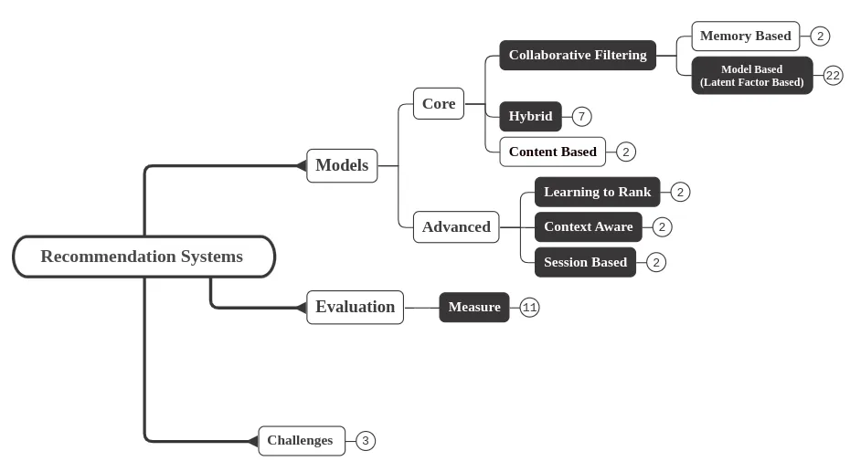
There have been a number of surveys and books focusing on the recommendation models developing different taxonomy of recommendation algorithms types. The popular recommendation systems hierarchy categorizes recommendation systems algorithms to collaborative filtering , content based and hybrid algorithms.

**Fig 7. The Popular Recsys Hierarchy in Literature**

As we can see there are two main approaches for collaborative filtering : memory-based and model-based.

Memory-based algorithm loads entire database into system memory and make prediction for recommendation based on such in-line memory database. It is simple but encounters the problem of huge data.

Model-based algorithm tries to compress huge database into a model and performs recommendation task by applying reference mechanism into this model. Model-based CF can response user’s request instantly.

Fore more infoemation about this taxonomy refer to my favorite article by Baptiste Rocca : “Introduction to recommender systems”.

Figure 8. presents an extended version of a well-established recommender systems taxonomy. This series will focus on model-based collaborative filtering, along with hybrid and advanced algorithms. The taxonomy has been constructed by analyzing original research papers and state-of-the-art solutions in recommender systems. Notably, it has been designed to minimize overlap between categories.

**Fig 8. Level #3 of Recommendation algorithms taxonomy(extended) . Mind-Map by author**

Latent factor models are a popular approach in recommender systems because they can capture hidden relationships between users and items without explicitly requiring all the user-item interactions. Following figure shows a breakdown of different subcategories and algorithms within this category.Notably Matrix factorization is the entire toolbox, representing the general concept of decomposing a matrix. SVD , ALS and PMF as well as MF variants for example are specific tools within that toolbox, each suited for a particular task within matrix factorization.

Notably , not all neural collaborative filtering (NCF) techniques are latent factor-based. However, many common NCF approaches do incorporate latent factors as a core concept. Here’s a breakdown:

NCF and Latent Factors:

Many NCF Models are Latent Factor-based: A significant portion of NCF research focuses on utilizing neural networks to model latent factors that capture user preferences and item characteristics. These latent factors are similar to those used in traditional matrix factorization techniques but learned through neural network architectures.
Examples of Latent Factor-based NCF: NeuMF (Neural Matrix Factorization), DeepFM (Deep Factorization Machine), and collaborative autoencoders are all examples of NCF models that leverage latent factors.
Not All NCF Models Rely on Latent Factors: While latent factors are prevalent, some NCF approaches might focus on directly modeling user-item interactions or relationships between item features through neural networks. These models wouldn’t necessarily involve the explicit extraction of latent factors.

Also Attention-based DCF (Deep Collaborative Filtering) can be both latent-based and non-latent-based, depending on the specific implementation.

we will update the taxonomy during this series , when we will be more familiar with models specification and attribution.

**Figure 9.** **Level #4 of Recommendation algorithms taxonomy(extended) . Mind-Map by author**

Most common and well-established (Core) algorithms

Matrix Factorization

Matrix factorization (MF) is a powerful technique used in collaborative filtering algorithms for building recommendation systems. It aims to decompose a user-item interaction matrix into two lower-dimensional matrices, capturing the underlying relationships between users and items.The main assumption behind matrix factorization is that there exists a pretty low dimensional latent space of features in which we can represent both users and items and such that the interaction between a user and an item can be obtained by computing the dot product of corresponding dense vectors in that space.

Matrix factorization relates to techniques to analyze and take advantages of rating matrix with regard to matrix algebra. Concretely, matrix factorization based CF aims to two goals. The first goal is to reduce dimension of rating matrix . The second goal is to discover potential features under rating matrix and such features will serve a purpose of recommendation. There are some models of matrix factorization in context of CF such as Latent Semantic Analysis (LSA), Latent Dirichlet Allocation (LDA), Principle Component Analysis (PCA), and Singular Value Decomposition (SVD).

Two serious problems in CF are data sparseness and huge rating matrix which cause low performance. When there are so many users or items, some of them don’t contribute to how to predict missing value and so they become unnecessary. In other words the rating matrix has insignificant rows or columns. Dimensionality reduction aims to get rid of such redundant rows or columns so as to keep principle or important rows/columns.

As result the dimension of rating matrix is reduced as much as possible. After that other CF approaches can be applied to the rating matrix whose dimension is reduced in order to make recommendation. Principle Component Analysis (PCA) is a popular technique of dimensionality reduction.

Matrix Factorization for Explicit Feedback

Matrix factorization is a latent factor model assuming that for each user u and item i there are latent vector representations pᵤ, qᵢ ∈ Rᶠ s.t. rᵤᵢ can be uniquely expressed — i.e. “factorized” — in terms of pᵤ and qᵢ. The Python library Surprise provides excellent implements of these methods.

The simplest idea is to model user-item interactions through a linear model. To learn the values of pᵤ and qᵢ, we can minimize a regularized MSE loss over the set K of pairs (u, i) for which rᵤᵢ is known. The algorithm so obtained is called probabilistic matrix factorization (PMF).

The loss function can be minimized in two different ways. The first approach is to use stochastic gradient descent (SGD). SGD is easy to implement, but it may have some issues because both pᵤ and qᵢ are both unknown and therefore the loss function is not convex. To solve this issue, we can alternatively fix the value pᵤ and qᵢ and obtain a convex linear regression problem that can be easily solved with ordinary least squares (OLS). This second method is known as alternating least squares (ALS) and allows significant parallelization and speedup.

The PMF algorithm was later generalized by the singular value decomposition (SVD) algorithm, which introduced bias terms in the model.

Matrix Factorization for Implicit Feedback

The SVD method can be adapted to implicit feedback datasets. The idea is to look at implicit feedback as an indirect measure of confidence. Let’s assume that the implicit feedback tᵤᵢ measures the percentage of movie i that user u has watched — e.g. tᵤᵢ = 0 means that u never watched i, tᵤᵢ = 0.1 means that he watched only 10% of it, tᵤᵢ = 2 means that he watched it twice. Intuitively, a user is more likely to be interested into a movie they watched twice, rather than in a movie they never watched. We therefore define a confidence matrix cᵤᵢ and a rating matrix rᵤᵢ as follows.

Matrix Factorization for Implicit and Explicit Feedback Both: Finally, the SVD++ algorithm can be used when we have access to both explicit and implicit feedbacks. This can be very useful, because typically users interact with many items (= implicit feedabck) but rate only a small subset of them (= explicit feedback). Let’s denote, for each user u, the set N(u) of items that u has interacted with. Then, we assume that an implicit interaction with an item j is associated with a new latent vector zⱼ ∈ Rᶠ. The SVD++ algorithm modifies the linear model of SVD by including into the user representation a weighted sum of these latent factors zⱼ.

It’s important to understand that listing “all” model based collaborative filtering for recommendation systems is difficult because research in this field is constantly evolving, and new variations and combinations of approaches emerge frequently. However, here’s a list encompassing some of the most common and well-established algorithms.

For deeper understanding of Matrix Factorization and its different variants you can refer to :

“Matrix Factorization Techniques for Recommender Systems”. Yehuda Koren, Robert Bell, Chris Volinsky. August 2009
James Le https://towardsdatascience.com/recsys-series-part-4-the-7-variants-of-matrix-factorization-for-collaborative-filtering-368754e4fab5

1. Alternating Least Squares (ALS):

ALS (Alternating Least Squares) is a popular matrix factorization technique widely used in collaborative filtering algorithms for recommendation systems. It excels in handling large and sparse datasets, making it a valuable tool for real-world scenarios.

[ — ] How it Works:

User-Item Interaction Matrix: Similar to other matrix factorization methods, we start with a user-item interaction matrix (R). Each row represents a user, each column represents an item, and each cell contains a value indicating the interaction between a user and an item (e.g., rating, purchase history).
Matrix Factorization: ALS decomposes this interaction matrix into two lower-dimensional matrices:

User Factor Matrix (U): This matrix has one row for each user and a smaller number of columns (k) representing the latent factors or features that influence user preferences.
Item Factor Matrix (V): This matrix has one row for each item and the same number of columns (k) as the user factor matrix. Each column represents the item features.

3. Iterative Optimization: Unlike other methods that optimize both matrices simultaneously, ALS takes an iterative approach:

Step 1: Fix the item matrix (V) and perform least squares regression to optimize the user matrix (U) that best approximates the product of U and Vᵀ to the user-item interaction matrix (R).
Step 2: Fix the user matrix (U) and perform least squares regression again, this time optimizing the item matrix (V) based on their product with U and their relation to the interaction matrix.

4. Predicting Ratings: Once the user and item factor matrices are learned, we can predict the missing interaction values (e.g., predict a user’s rating for an item they haven’t interacted with) by multiplying the corresponding rows in the user and item factor matrices:

Predicted Rating = U_i * V_jᵀ

[ — ] Benefits of ALS:

Scalability: ALS efficiently handles large and sparse datasets, making it suitable for real-world recommendation systems with millions of users and items.
Computational Efficiency: The iterative approach allows for efficient computation, particularly compared to techniques that update both matrices simultaneously.
Parallelization: ALS can be easily parallelized, further improving its efficiency on large datasets.
Regularization: It naturally incorporates regularization by minimizing the sum of squared errors, which helps prevent overfitting.

[ — ] Limitations of ALS:

Non-negativity: Unlike NMF, the factors in ALS are not constrained to be non-negative, which can be a limitation for data where interaction values are inherently positive (e.g., ratings).
Cold Start Problem: Similar to other matrix factorization methods, ALS can struggle with recommending items to new users or items with limited interaction history.

[ — ] Variations and Extensions:

Weighted ALS: This incorporates user and item weights to prioritize specific users or items based on their importance or reliability.
Time-aware ALS: This integrates temporal information by adding time-related features to the user and item matrices, allowing for recommendations that adapt to evolving user preferences.
Hybrid ALS: This combines ALS with other techniques, such as content-based filtering or knowledge graph embeddings, to leverage additional information and improve recommendation accuracy.

Singular Value Decomposition (SVD):

Singular Value Decomposition (SVD) is a dimensionality reduction technique commonly used in recommender systems for making personalized recommendations. SVD was first used by Billsus and Pazzani in 1998 in recommendation service. They explored a few machine learning algorithms for collaborative filtering tasks and identified SVD as the best-performing one.

Imagine you have a dataset representing user interactions with items, typically in the form of a matrix. This matrix has rows representing users and columns representing items. Each cell contains the rating (e.g., preference score) a user gave to an item, or it might be left blank if there’s no interaction.

This user-item rating matrix can be very high dimensional, especially if you have a large number of users and items. SVD helps reduce this dimensionality while capturing the important underlying structure of the data.

[ — ] How SVD Works

Decompose the Matrix: SVD decomposes the user-item rating matrix (A) into three smaller matrices:
U: A left singular vectors matrix representing user latent factors.
Σ (Sigma): A diagonal matrix containing the singular values, which capture the importance of each latent factor.
V^T (Transposed Right Singular Vectors): A right singular vectors matrix representing item latent factors.

[ — ] Latent Factors

Latent factors are hidden variables that capture the underlying preferences or characteristics of users and items.
For users (U), these factors might represent genres they prefer, preferred brands, or browsing patterns.
For items (V^T), these factors might represent the genre, topic, style, or brand of the item.

[ — ] Making Recommendations

By multiplying the reduced-dimensionality matrices (U containing user factors and Σ containing singular values), we can estimate the missing ratings or predict how a user might rate an unseen item. This estimated rating matrix helps recommend items to users based on their inferred preferences (latent factors) and the relationships between items through the latent factors.

[ — ] Cons and pros of SVD

Advantages:

Mathematically well-understood and stable.
Effective for capturing global patterns in the data.

Disadvantages:

May not be as efficient for large datasets.
Limited ability to capture complex non-linear relationships between users and items.

You can find more details about SVD and variants and Surprise implementation of SVD in my github.

2. Non-Negative Matrix Factorization (NMF)

At its core, NMF is a matrix factorization technique similar to Singular Value Decomposition (SVD). However, it imposes an important constraint: all elements in the factorized matrices must be non-negative. This aligns nicely with common recommendation scenarios where interactions like ratings, view durations, or purchases are inherently non-negative. Then NMF decomposes this matrix into two lower-dimensional matrices:

User Factor Matrix (U): Each row represents a user, and each column represents a latent factor or feature. These factors describe the underlying preferences or characteristics of a user.
Item Factor Matrix (V): Each row represents an item, and each column represents the same latent factors from the user factor matrix. These factors quantify how strongly an item aligns with a particular preference.

The original user-item matrix can be approximated by the product of the two factor matrices:

User-Item Matrix ≈ U * Vᵀ

To predict a user’s potential interest in an item they haven’t interacted with yet, we multiply their corresponding row in the user matrix (U) with the item’s column in the item matrix (V). Higher predicted values indicate a stronger likelihood of that user having a positive interaction with the item.

import pandas as pd
import numpy as np
from sklearn.decomposition import NMF

V = np.array([[0,1,0,1,2,2],
              [2,3,1,1,2,2],
              [1,1,1,0,1,1],
              [0,2,3,4,1,1],
              [0,0,0,0,1,0]])

V = pd.DataFrame(V, columns=['John', 'Alice', 'Mary', 'Greg', 'Peter', 'Jennifer'])
V.index = ['Vegetables', 'Fruits', 'Sweets', 'Bread', 'Coffee']

nmf = NMF(3)
nmf.fit(V)

H = pd.DataFrame(np.round(nmf.components_,2), columns=V.columns)
H.index = ['Fruits pickers', 'Bread eaters',  'Veggies']

W = pd.DataFrame(np.round(nmf.transform(V),2), columns=H.index)
W.index = V.index

reconstructed = pd.DataFrame(np.round(np.dot(W,H),2), columns=V.columns)
reconstructed.index = V.index

[ — ] Advantages:

Non-negativity: The non-negativity constraint aligns well with real-world recommendation scenarios where data is usually positive (ratings, purchases, etc.). This makes the results more interpretable.
Part-based representation: NMF learns "parts" that can be combined to explain the whole. Imagine latent features or factors representing genres in a movie recommendation system. Each user will have different affinities for these genres, and each movie will be a combination of them.
Sparsity Handling: NMF works well with sparse datasets, which is typical in recommendation systems where users have interactions with only a small fraction of the total items.
Computational Efficiency: Relative to some other methods, NMF can be computationally efficient for large datasets.

[ — ] Limitations:

May not capture as much information as SVD due to the non-negativity constraint.
Sensitive to initialization and can get stuck in local optima during optimization.

**Fig 11. NMF, SVD, SVD++. SlopOne with surprise on MovieLense data, Author Code**

You can find more core algorithms implementation in my github repo on Book-Crossing dataset (available on my kaggle datasets) .

3. Probabilistic Matrix Factorization (PMF):

PMF is a specific type of matrix factorization designed for collaborative filtering in recommendation systems. It builds upon the concepts of SVD but incorporates a probabilistic model. The assumption is ratings are generated from a latent factor model where users and items are associated with latent factors and ratings are subject to noise and uncertainty.

In fact PMF is a matrix factorization technique based on probabilistic models, designed to handle the uncertainty and noise inherent in recommendation system data. It assumes that user preferences and item characteristics can be represented by latent factors, but it models them as probability distributions rather than fixed points.

[ — ] How PMF Works

User-Item Matrix: As with other matrix factorization methods, we start with a partially observed user-item interaction matrix (R), where rows represent users, columns represent items, and each cell contains a rating, purchase record, or another interaction measure.
Latent Factor Matrices: PMF assumes Gaussian distributions for both user and item latent factors:

User Factor Matrix (U): Each row represents a user. Each column represents a latent factor (feature) modeled as a Gaussian distribution with zero mean and a user-specific variance.
Item Factor Matrix (V): Each row represents an item. Each column represents a latent factor (feature) modeled as a Gaussian distribution with zero mean and an item-specific variance.

3. Probabilistic Modeling: PMF models the observed ratings (elements in matrix R) as a conditional probability distribution. It assumes that the observed rating for a user-item pair depends on a user’s latent factors, the item’s latent factors, and some Gaussian noise.

4. Model Learning: The goal of PMF is to learn the parameters of the user and item factor distributions (means and variances) that maximize the likelihood of the observed data. This is typically done using an algorithm like Maximum a Posteriori (MAP) estimation or gradient descent-based optimization methods.

5. Recommendations: After learning the model, to estimate the rating a user would give to an item, we take a dot product of the user’s latent factors and the item’s latent factors and account for the expected noise. The higher the predicted rating, the more likely the user finds the item interesting.

[ — ] Advantages of PMF

Uncertainty Handling: PMF’s probabilistic treatment makes it robust to noise and outliers in the data. This is crucial since rating data can often be inconsistent.
Flexibility: The probabilistic framework allows for extensions, such as incorporating implicit feedback (e.g., viewing time, clicks) and side information (user demographics, item content).
Good Performance: PMF has demonstrated strong performance on various recommendation tasks, often outperforming simpler matrix factorization methods.

[ — ] Limitations and Considerations

Computational Cost: PMF can be computationally more expensive than some basic matrix factorization methods, especially for large datasets.
Parameter Tuning: The performance of PMF can be sensitive to hyperparameter settings.

[ — ] Extensions

To enhance PMF models and overcome limitations, several extensions have been developed:

Incorporating time dynamics: Modeling how user preferences change over time can improve recommendation accuracy.
Handling bias: Accounting for user-specific and item-specific biases (e.g., rating tendencies) can refine the results.
Social PMF: Integrating social network information with PMF can leverage trust and social connections to enhance recommendations.

For more details about PMF refer to Oscar Contreras Carrasco article PMF for Recommender Systems

5. Biased Matrix Factorization (BMF):

BMF extends matrix factorization by incorporating user and item biases alongside explicit feedback data.

[ — ] Bias modeling:

User bias: Captures a user’s general tendency to rate items higher or lower on average, independent of the specific item.
Item bias: Reflects the inherent popularity of an item, independent of individual user preferences.

[ — ] Benefit: Allows the model to better distinguish between genuine user preferences and general rating tendencies, potentially leading to more accurate recommendations based on explicit feedback.

6. Matrix Factorization with Side Information: MF can be limited by only considering user-item interaction data. Matrix Factorization with Side Information (MF-SI) addresses this limitation by incorporating additional information about users, items, or the context of interactions.

Side information refers to additional data that can enrich the user-item interaction matrix. This information can be:

User-based: Demographics, interests, preferences (e.g., age, occupation, genre preferences)
Item-based: Features, attributes, categories (e.g., movie genre, book author, product category)
Contextual: Time, location, specific circumstances of interaction (e.g., day of the week, time of day, occasion)

7. Weighted Matrix Factorization: Assigns different weights to implicit and explicit feedback based on their perceived reliability.

8. Matrix Factorization with Temporal Features: Matrix Factorization often assumes that user preferences and item characteristics are static over time. This limitation can be addressed by incorporating temporal features into the model, leading to Matrix Factorization with Temporal Features (MF-TF).

9. Hybrid Matrix Factorization: Combines different types of matrix factorization techniques tailored for various data modalities within a single framework.

10 . MF-Implicit

While the term “MF-implicit” suggests a focus on implicit feedback data, it still falls under the umbrella of Matrix Factorization techniques for recommender systems. While MF-implicit itself isn’t a specific algorithm, it refers to adapting Matrix Factorization (MF) techniques to handle implicit feedback data like clicks, views, or purchases. Here are some algorithms that fall under the “MF-implicit” umbrella:

BPR (Bayesian Personalized Ranking): Introduced earlier, BPR can be applied to implicit feedback data. It focuses on learning an item ranking, aiming to rank items higher that a user has interacted with compared to un-interacted-with ones.
Collaborative Matrix Factorization with Implicit Feedback (CMF-Implicit): This technique adapts traditional Collaborative Matrix Factorization (CMF) to implicit feedback by by: Modeling item popularity: Accounts for the inherent attractiveness of items independent of user preferences and Incorporating negative sampling: Creates artificial negative interactions (items the user likely hasn’t interacted with) for training the model.
Probabilistic Matrix Factorization (PMF) with Implicit Feedback: PMF can be adapted for implicit feedback by: Utilizing a specific loss function suited for implicit data, like logistic loss or negative log-likelihood and Incorporating negative sampling similar to CMF-Implicit.
Matrix Factorization with Confidence-Weighted Item Popularity (MF-CWIP): This technique aims to improve recommendations by Modeling item popularity with confidence weights and Assigning higher weights to items with a stronger implicit signal (e.g., frequent clicks) compared to less informative interactions.
Auxiliary Information Matrix Factorization (AIMF) with Implicit Feedback: Similar to standard AIMF, this approach incorporates side information like user demographics or item attributes alongside implicit interactions into the latent factor learning process.

Model Selection

Selecting the most suitable matrix factorization (MF) algorithm for your recommendation system requires careful consideration of several factors. Here’s a breakdown of key aspects to guide your choice:

1. Data Characteristics:

[ — ] Feedback Type:

Explicit Feedback (Ratings): If you have explicit user ratings (stars, thumbs up/down), algorithms like Standard MF (SVD) or Probabilistic MF (PMF) can be effective.
Implicit Feedback (Clicks, Views): Algorithms designed for implicit feedback like MF-Implicit, which models item popularity and incorporates negative sampling, are better suited.
Combination: If you have both explicit and implicit feedback, consider PMF (can handle both), Weighted MF (assigns weights based on perceived reliability), or even hybrid approaches combining MF techniques with other methods.

[ — ] Data Sparsity: The amount of missing values in the user-item interaction matrix. Sparse data can be challenging for some algorithms.

SVD and PMF: Might struggle with sparse explicit rating data.
MF-Implicit: Designed specifically to handle sparse implicit feedback data.
NMF: Can be useful for sparse data due to its non-negative constraints, but limited in handling explicit feedback with negative values.

[ — ]Side Information Availability: Do you have additional data like user demographics or item features?

MF-Side Information: Integrates side information alongside user-item interactions to potentially enrich the model’s understanding.

2. Application Requirements:

[ — ] Accuracy: How important is it for the recommendations to be highly accurate?

SVD, PMF, and BMF: Generally perform well in terms of accuracy.
MF-Implicit: Might require additional tuning for accuracy with implicit feedback data.

[ — ] Interpretability: Do you need to understand the reasoning behind the recommendations?

SVD and NMF: Offer interpretable latent factors that can reveal user preferences and item characteristics.
PMF, BMF, and MF-Implicit: Might be less interpretable due to their probabilistic or implicit feedback handling mechanisms.exclamation

[ — ] Scalability: How large is your dataset, and how many users and items do you need to handle?

SVD and PMF: Generally scalable for large datasets.
NMF: Efficient for large datasets due to its non-negative factorization.
MF-Implicit and BMF: Might require more computational resources depending on the specific implementation.

[ — ]Cold Start Problem: How well should the system handle new users or items with limited data?

SVD and PMF: Might struggle with cold start for new users/items.
MF-Implicit: Can potentially handle cold start for items with implicit feedback data.
Hybrid approaches: Combining MF with content-based filtering (utilizes item features) can help address cold start for items.

3. Additional Considerations:

Real-time vs. Offline Recommendations: If you need real-time recommendations, consider the computational efficiency of the algorithm.
Domain-specific Knowledge: Can you leverage domain-specific knowledge to guide your choice? For example, in a movie recommendation system, you might prioritize algorithms that can handle time-sensitivity of movie preferences.

Here’s a table summarizing some key considerations for choosing an MF algorithm:

**Fig 12 . How to Choose the most suitable matrix factorization algorithms, table by author**

Brief History of Recommendation Systems

Figure 13. shows my gathering of recommendation algorithms history and evolution. The critical points of the time line is as bellow:

**Fig 13. History of Recommendation Systems, Figure by author**

[ — ] Early Days (1990s):

Simple Beginnings: Recommendation systems relied on rule-based algorithms (e.g., “If a user buys horror, recommend similar movies”) and content-based algorithms (e.g., recommend books based on genre or author) that utilized predefined rules or item features.
Limitations: These approaches faced challenges with scalability, data sparsity (limited user-item interaction data), and the cold start problem (difficulty in recommending for new users or items).

[ — ] Collaborative Filtering (CF) Era (2000s):

A Paradigm Shift: CF algorithms, like K-Nearest Neighbors (KNN) and Matrix Factorization (MF) variants (User-based MF, Item based MF), revolutionized the field.

UMF/IMF and memory-based collaborative filtering (CF) are different approaches to building recommendation systems, although they share some similarities.

User-based Matrix Factorization (UMF):

Concept: UMF focuses on finding similar users based on their interaction patterns.
Process: 1)User-item interaction matrix is used as input. 2) The matrix is transposed, effectively swapping users and items.3 ) Regular MF techniques (like SVD) are applied to the transposed matrix. 4) The resulting factors represent user latent factors, capturing user preferences.
Recommendations: 1) To recommend items for a user, we find the k nearest neighbors (most similar users) based on their user latent factors. 2) We then recommend items that these similar users have interacted with and the target user hasn’t.

Item-based Matrix Factorization (IMF):

Concept: IMF focuses on finding similar items based on their interaction patterns with users.
Process: User-item interaction matrix is used directly. Regular MF techniques (like SVD) are applied to the original matrix. The resulting factors represent item latent factors, capturing item characteristics.
Recommendations: To recommend items for a user, we consider their past interactions and identify items with similar latent factors (characteristics) to those items they have interacted with.

Leveraging User Data: These algorithms analyzed user-item interaction data (purchases, ratings, etc.) to identify similar users or items and recommend items enjoyed by similar users but not interacted with by the target user.

Benefits: CF offered improved accuracy and addressed the cold start problem to a certain extent.

[ — ] Content-based Filtering (CBF) Integration (2000s-2010s):

Enriching Recommendations: CF was combined with CBF techniques to incorporate both user preferences and item characteristics.

Example: CF could be combined with content-based similarity measures to recommend movies similar to what a user watched before, while also considering their past preference for specific actors or directors.

Benefits: This hybrid approach led to more diverse and personalized recommendations.

[ — ] Matrix Factorization (MF) and Beyond (2010s-present):

Extracting Hidden Patterns: Advanced MF techniques like Singular Value Decomposition (SVD) and Non-negative Matrix Factorization (NMF) further refined MF by capturing latent factors (hidden features) from user-item interaction data.

Model-based CF: Introduction of advanced models like SVD++ (extension of SVD) and neighborhood-based methods (improved KNN variants) further enhanced personalization.

Deep Learning Models: The emergence of Recurrent Neural Networks (RNNs) and Convolutional Neural Networks (CNNs) opened new avenues for handling complex user-item interactions and sequential data (e.g., purchase history).

[ — ] Factorization Machines (FM) and FFM (2010s- present):

Addressing Limitations of MF: FM introduced interaction terms to capture how user preferences for one feature can be influenced by another, addressing a limitation of MF that assumed feature independence.

FFM (Field-aware Factorization Machines) further enhanced feature interactions by introducing field-specific latent factors, allowing the model to learn interactions based on feature categories.

[ — ] Emerging Trends:

Explainability & Transparency: Techniques like LIME are being employed to make complex models interpretable and build user trust.

New Data Sources: Algorithms are being adapted to utilize diverse user data like social media activity, browsing behavior, and real-time context for more comprehensive and context-aware recommendations.

Addressing Ethical Concerns: Fair recommendation algorithms are being developed to ensure fairness and avoid bias in recommendations.

This journey showcases the continuous pursuit of personalized and accurate recommendations. As AI and data analysis techniques evolve, we can expect even more sophisticated and impactful recommendation systems shaping the future of how we interact with information and products online like LLM based recommendation systems:

[ — ] Large Language Models (LLMs):

Large Language Models (LLMs) are transforming the landscape of recommendation systems, offering innovative ways to personalize user experiences. This survey delves deeper into LLM-based recommendation approaches and explores how they leverage the power of LLMs for enhanced recommendations.

Figure from paper :Harnessing the Power of LLMs in Practice: A Survey on ChatGPT and Beyond

Understanding User Preferences through Textual Data:

Unlike traditional methods that rely solely on ratings or purchase history, LLMs can process textual user data like:

Reviews: LLMs can analyze user reviews of products or services to comprehend user preferences, opinions, and pain points. This allows them to go beyond explicit ratings and capture nuanced sentiment and specific aspects users value.
Search queries: By understanding the language used in user search queries, LLMs can infer user interests and preferences. Identifying keywords, synonyms, and related search terms helps create a more comprehensive profile of what users are actively seeking.
Social media interactions: Analyzing user behavior on social media platforms, such as posts, comments, and shares, reveals valuable insights into user preferences and interests. LLMs can process this textual data to understand user sentiment towards specific products, brands, or topics.

Enhanced Content Representation with LLMs:

LLMs excel at processing and understanding textual descriptions of items, such as:

Product descriptions: By analyzing product descriptions, LLMs can extract key features, functionalities, and benefits. This allows them to create richer and more informative item representations compared to traditional methods that rely solely on keywords or product categories.
Article summaries: LLMs can process lengthy articles or news items and generate concise summaries highlighting key points and relevant information. This enables them to recommend articles tailored to user interests and attention spans.
Movie synopses: LLMs can analyze movie synopses to understand plot elements, genres, and themes. This allows them to recommend movies based not just on user ratings or similar genres but also on their specific taste in plotlines, characters, or thematic elements.

[ — ] LLM-Based Recommendation Approaches(2018 - present):

Large Language Models (LLMs) have emerged as powerful tools in the field of Natural Language Processing (NLP) and have recently gained significant attention in the domain of Recommendation Systems (RS). These models, trained on massive amounts of data using self-supervised learning, have demonstrated remarkable success in learning universal representations and have the potential to enhance various aspects of recommendation systems by some effective transfer techniques such as fine-tuning and prompt tuning, and so on. The crucial aspect of harnessing the power of language models in enhancing recommendation quality is the utilization of their high-quality representations of textual features and their extensive coverage of external knowledge to establish correlations between items and users. Likang Wu et al. categorized these models into two major paradigms, respectively Discriminative LLM for Recommendation (DLLM4Rec) and Generative LLM for Recommendation (GLLM4Rec), with the latter being systematically sorted out for the first time.

**Fig 14.** **A taxonomy of the research for large language models on recommendation systems**

Discriminative LLM-based Recommendation (DLLM4Rec):

Example 1: Imagine a system that recommends books based on user reviews and book descriptions.

An LLM can be trained on a dataset of user reviews and corresponding book ratings.
The LLM learns to analyze user reviews and book descriptions, extracting key features and user preferences.
Based on this understanding, the LLM predicts a rating for a specific book for a given user, allowing the system to recommend highly rated books based on the user’s review history and inferred preferences.

Example 2: An e-commerce platform uses an LLM to analyze user search queries for clothing and product descriptions.

The LLM understands the user’s search intent by analyzing keywords and related terms in the query.
It then matches this information with relevant product descriptions, considering features, styles, and user preferences.
The LLM recommends clothing items that closely align with the user’s search intent and inferred preferences from their search behavior.

2. Generative LLM-based Recommendation (GLLM4Rec):

Example 1: A news aggregator utilizes an LLM to generate personalized news summaries based on user interests.

The LLM is trained on a vast corpus of news articles and user interactions (e.g., clicks, reading time) to understand user preferences for specific topics.
When a new user signs up, the LLM personalizes their news feed by generating summaries of articles relevant to their interests.
This allows users to quickly grasp the gist of relevant news stories and efficiently discover content they’ll enjoy.

Example 2: A travel platform employs an LLM to generate personalized trip itineraries based on user preferences and travel destination information.

The LLM analyzes user reviews and travel blogs about the destination, extracting information about activities, attractions, and preferred travel styles.
Based on this understanding and the user’s preferences, the LLM generates a personalized itinerary suggesting activities, restaurants, and points of interest that align with their interests.

LLM-BRs Looking Forward: Challenges and Opportunities:

While LLM-based recommendations hold immense potential, challenges remain:

Data sparsity and cold-start problem: LLMs require vast amounts of training data, which can be a limitation in specific domains. Techniques like transfer learning and prompt engineering can mitigate this.
Explainability and bias mitigation: Addressing concerns around the explainability and potential biases of LLMs is crucial. Research efforts are underway to improve transparency and develop fair recommendation algorithms.
Combining LLMs with other techniques: Hybrid approaches combining LLMs with traditional methods (CF, CBF) can leverage the strengths of both, leading to more robust and personalized recommendations.

Classic Recommendation Algorithms (practically effective)

In this section , we will introduce a different look of some kinds of practical recommendation models chronologically.

**Fig 15. Rise of Matrix Factorization based algorithms**

The models are selected mainly based on two principles:

The model has important effect on the progress of recommender system,
The model has been successfully deployed on the products.

**Fig 16. First wave : Classic recommendation models evolution, Image extended by author from origin**

**Fig 17. First wave : Classic recommendation models evolution (combining MF with regression)**

Factorization Machine

Factorization Machines (FM) are an extension of Matrix Factorization, offering more flexibility by capturing interactions between latent factors associated with different features.

Paper: https://arxiv.org/pdf/2203.11026.pdf

Code (Tensorflow): https://github.com/babakx/fm_tensorflow/blob/master/fm_tensorflow.ipynb

Code (PyTorch): https://medium.com/@datadote/factorization-machines-pictures-code-pytorch-9fca1c300838

Explanation:

Core Idea: FM assumes that the user’s preference for an item can be determined not just by individual features (user ID, item ID) but also by how these features interact with each other.
Matrix Factorization Recap: MF decomposes the user-item interaction matrix into user and item latent factors, allowing for predicting ratings based on dot products of these factors.
FM Improvement: FM introduces an additional term that captures pairwise interactions between latent factors of different features. This allows the model to learn how user and item combinations influence preferences.

Core Components:

Latent Factors: FMs represent each feature with a low-dimensional latent vector.expand_more These vectors capture hidden concepts associated with the feature.
Pairwise Interactions: The model computes the element-wise product of the latent vectors for each pair of features.expand_more
Inner Product: The element-wise products are then summed to obtain a score for each feature interaction.
Linear Model: In addition to interaction terms, FMs also include a linear term that models the individual effects of each feature.
Prediction: The final prediction is a linear combination of the interaction terms and the linear term.

Benefits of FMs:

Improved Accuracy: By capturing feature interactions, FMs can achieve better prediction accuracy compared to linear models, especially when complex relationships exist between features.
Flexibility: FMs can handle various feature types (categorical, numerical) without explicit feature engineering.exclamation
Scalability: FMs are efficient in terms of training time and memory usage, especially for sparse datasets with many features.expand_more

Limitations of FMs:

Higher Order Interactions: While FMs capture pairwise interactions, they don’t inherently capture higher-order interactions (involving more than two features).
Interpretability: Understanding the contribution of specific feature interactions can be challenging compared to simpler models.

Comparison with Matrix Factorization (MF):

Both techniques address the sparsity problem in collaborative filtering.
MF focuses on decomposing the user-item rating matrix into two lower-dimensional matrices, capturing user and item latent factors.expand_more
FM leverages pairwise interactions between features, potentially capturing richer information about user preferences and item characteristics.

And for full search of FM variants and original paper you can follow the links in the bellow table . I will explain some of deep based algorithms in Part 2. of this series.

For a consistent implementation if you want to use open sources packages i recommend you to apply pytorchFM and example codes in github

2. Field Aware Factorization Machine

FFM (Field-aware Factorization Machines) is a powerful algorithm for recommendation systems, extending Matrix Factorization (MF) by capturing interactions between latent factors associated with different features.

Field-aware Factorization Machines (FFMs) are a machine learning model specifically designed for recommender systems and other classification tasks involving categorical data. They address limitations of traditional Factorization Machines (FMs) by incorporating field information for improved performance.

Paper: https://www.csie.ntu.edu.tw/~cjlin/papers/ffm.pdf

Challenges with Factorization Machines (FMs):

FM Limitations: Standard FMs treat all features equally, regardless of the field they belong to (e.g., user ID, movie genre, director). This might not capture the inherent relationships between features from different fields effectively.
Example: A user who likes action movies by a specific director might also be interested in other action movies by different directors. A standard FM might struggle to capture this nuanced relationship.

FFMs to the Rescue:

Field-awareness: FFMs introduce the concept of “fields.” Each feature belongs to a specific field, providing the model with additional context.In a movie recommendation system, fields might include “user ID,” “movie genre,” “director,” “actor,” etc.

How FFMs Work:

Feature Representation: Like FMs, FFMs represent features as dense embedding vectors. Here, however, separate embedding vectors are learned for each field.
Pairwise Interactions: FFMs consider pairwise interactions between features. However, the interaction strength now depends on the fields the features belong to.
Field-aware Interaction: FFMs introduce a field-aware interaction term that modulates the interaction strength based on the fields of the interacting features. This allows the model to capture more nuanced relationships between features from different fields.

Benefits of FFMs:

Improved Feature Interaction Modeling: By considering field information, FFMs can capture more precise relationships between features, leading to better prediction accuracy.
Sparse Data Efficiency: FFMs work well with sparse data (common in recommender systems) due to their use of embedding vectors.
Interpretability: To some extent, FFMs offer better interpretability compared to complex deep learning models, as feature interactions can be analyzed based on field information.

Applications of FFMs:

Recommender Systems: FFMs excel at recommending items to users by capturing user preferences and item characteristics based on different fields (e.g., user demographics, genre, director).
Click-through Rate (CTR) Prediction: FFMs are useful in online advertising to predict the likelihood of a user clicking on an ad based on user attributes, ad content, and context (e.g., device, time of day).
E-commerce Personalization: FFMs can personalize product recommendations and search results on e-commerce platforms based on user purchase history and product .

Some of open sources you can use to test FFM are: libFFM and pytorchFM. Also you can find more details about the algorithm and an implementation with xLearn, here.

3. FTRL

While FTRL (Follow the Regularized Leader) is not commonly used as the core algorithm for recommendation systems due to its limitations in capturing complex user-item interactions, it can be employed as an optimization technique for training certain models. Here’s an example demonstrating its use with Logistic Regression for recommendation:

import torch
import torch.nn as nn
from torch.optim import FTRL

# Sample user-item interaction data (replace with your actual data)
users = torch.tensor([1, 2, 3, 1, 2])
items = torch.tensor([2, 1, 4, 3, 2])
ratings = torch.tensor([1, 0, 1, 0, 1])

class LogisticRegression(nn.Module):
  def __init__(self, num_users, num_items, embedding_dim):
    super(LogisticRegression, self).__init__()
    self.user_embedding = nn.Embedding(num_users, embedding_dim)
    self.item_embedding = nn.Embedding(num_items, embedding_dim)
    self.linear = nn.Linear(embedding_dim * 2, 1)

  def forward(self, user_id, item_id):
    user_embedding = self.user_embedding(user_id)
    item_embedding = self.item_embedding(item_id)
    x = torch.cat([user_embedding, item_embedding], dim=-1)
    return torch.sigmoid(self.linear(x))

Training with FTRL:

# Hyperparameters
learning_rate = 0.1
alpha = 0.1
beta = 1.0
l1 = 0.0

model = LogisticRegression(users.max() + 1, items.max() + 1, 10)
optimizer = FTRL(model.parameters(), alpha=alpha, beta=beta, l1=l1, lr=learning_rate)

# Training loop (adjust epochs and loss function as needed)
for epoch in range(10):
  for i in range(len(users)):
    user_id, item_id, rating = users[i], items[i], ratings[i]
    predicted_rating = model(user_id, item_id)
    loss = nn.BCELoss()(predicted_rating, rating.float())

    optimizer.zero_grad()
    loss.backward()
    optimizer.step()

    # Print training progress (optional)
    if i % 100 == 0:
      print(f"Epoch {epoch+1}, Batch {i+1}/{len(users)}, Loss: {loss.item():.4f}")