A separate guide for separable convolutions

I was working on an object detection problem some time ago when I came to know about a state-of-the-art CNN architecture for object detection problems called “Mobilenet”.
Mobilenet is an extremely lightweight model mostly used for implementing computer vision on mobile devices. But what makes this CNN architecture special is something known as separable convolution layers. These separable convolutions can reduce the number of trainable parameters in convolution layers up to 90%.
Majorly, two types of separable convolutions are quite popular among the community.
· Spatially separable convolutions
· Depthwise separable convolutions
Spatially separable convolutions
Before starting about spatially separable convolutions, we should first understand what “spatial” means in general.
Anything which is relating to any other object spatially means that the positions of these two objects play an important role. Think about any image, the pixels in this image are in a spatial relationship with each other. If I interchange some of the pixels here and there then the image will lose its meaning. Also if I convert this image to an array and then flatten that array, then the spatial information in that image is lost. (This phenomenon is called spatial loss, which is why people came up with convolution layers in the first place).
Spatial convolutions spit the dimensions of the kernel and then perform the convolution operation one by one on the image. Suppose if we have the image, instead of applying any kernel of 3✖3 sizes, we separate this kernel into 2 kernels of size 3✖1 and 1✖3 and then apply convolution.


By doing this we can reduce the number of convolutions from 9 to 6 and thus reducing the expense, But this technique isn’t very useful in most cases, the reason being that these types of convolutions can’t capture complex features
Depthwise separable convolutions
These types of convolutions were the major area of interest for scientists in mobile net architecture.
Let’s think of any image of size 7✖7✖3 and kernels of size 3✖3✖1. if we want to increase the number of channels from 3 to 256, then mostly we use 256 kernels of size 3✖3 on top of the image and stack them together to create a feature map of dimensions 5✖5✖256. But in depthwise convolution, we split this into 2 parts.
First, we shrink the height and width of the image by keeping the channels the same, then we increase the number of channels by making height and width constant
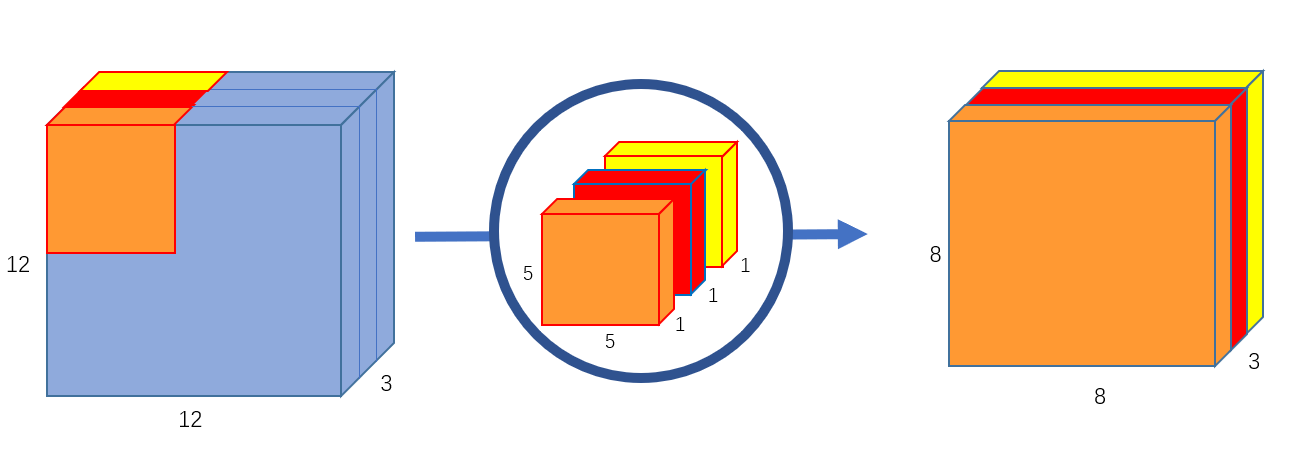
Part1- constant channels
Let’s take the above example only we have an image of size 7✖7✖3. We will do convolution with 3 kernels of size 3✖3✖1. It will give us a feature map of 5✖5✖3

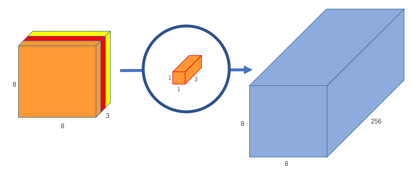
Part2- constant height and width
Now we will take 256 kernels of size 1✖1 and convolve it with the intermediate feature map of size 5✖5✖3, which we got in the 1st part. It will give us the feature map of size 5✖5✖256 because 1✖1 kernels don’t reduce the size of the input.

You must be thinking why do we need this, we can easily achieve the above feature map in one step only by using 256 kernels of size 3✖3. The reason is efficiency. Let us calculate the number of multiplications our computer has to do in both cases.
In simple convolution, the number of multiplications would be 7*7*3*3*3*256, equal to 338,688. Now in the depthwise separable convolution, the total number of multiplications would be 7*7*3*3*3*3 for the constant channel part and 5*5*3*1*1*256 for the constant height and width section. So, the total multiplications in the depthwise convolution will be 23,169, which is only 6.84% of the above method.
One thing to remember here is that these separable techniques don’t work on the Fully connected layers. also, here we increased the number of channels from 3 to 256 in just one convolution in real-world scenarios we gradually increase the number of channels. So, the techniques may or may not give such a magnificent reduction in the calculation (here, it gave 100–6.84 = 93.16% reduction)
References
- https://towardsdatascience.com/a-basic-introduction-to-separable-convolutions-b99ec3102728
- https://towardsdatascience.com/a-comprehensive-introduction-to-different-types-of-convolutions-in-deep-learning-669281e58215
- https://paperswithcode.com/method/depthwise-separable-convolution
- https://paperswithcode.com/method/mobilenetv1
And this concludes my discussion for separable convolutions. There is much more to this and I have only scratched the surface of it. If you want to know more about separable convolutions, I have given links to the article and research papers I referred to, while writing this article. Thank you if you are reading till here :).
