Deep Learning, NeuroEvolution & Extreme Learning Machines

In our previous tutorial we introduced Deep Learning (DL) and tried to understand Artificial Neural Networks (ANNs) in more detail: particularly focusing on deep feed forward neural nets (FFNNs), a.k.a. Multi-Layered Perceptrons (MLPs).
We ended by training one to paint a simple picture

In this second tutorial on Deep Learning, we shall try to get a better understand of how Neural Networks learn

Let us assume that all problems, no matter how complex, can be codified as some set of values (x) that get transformed into some other set of values (y).
input (x) → output (y)
Now these values may be numerical: e.g. pixel x-y coordinates: x = (1,1) → RGB colour values: y = (225,225,225)

These values could even be symbolic, e.g. x = “of course john has fun with the game” → y = “natuerlich hat john spass am spiel”.

But in the end, there are some input values (x) which turn into some output values (y). Initially, Artificial Intelligence (AI) research focused heavily on symbolic rules to define how these inputs (x) should be changed into the desired outputs (y).

This was a fine start and worked for the most part, but codifying rules requires expertise of that specific domain and research started turning toward automating this time-consuming part and Machine Learning (ML) methods were developed to learn these rules automatically (e.g. Inductive Logic Programming ILP).

Of course, why limit ourselves to learning only symbolic rules? We could think of a “rule” as a mathematical function (y = f( x ) ) that transforms a particular input value (x) into a desired output value (y).


In fact, by remodelling the problem as a non-symbolic one, we suddenly have a wealth of numerical algorithms developed in fields outside of AI and Computer Science (e.g. linear regression borrowed from statistics or multi-agent systems borrowed from complexity science, etc).

Deep Learning (DL) is currently one of the most popular ML methods which uses Deep Neural Networks to learn any mathematical function

So how exactly does a Neural Network learn a function?
In our previous post, you may have noted that each neuron already includes a simple function (e.g. sigmoid, tanh, relu, etc).

A neuron’s function can never change its core shape, rather it is simply rotated, shifted and stretched (by adjusting the neuron’s weights and bias values — which act as the function’s parameters).

Therefore, it is the parameters of functions we are learning (e.g. the bias and weights of each neuron). This is why in practise, deep learning boils down to adjusting the bias and weights of neurons.

The simple sigmoid or relu functions of neuron get combined (via the multi-layered neural network architecture) to approximate more complicated function shapes

Even learning extremely complicated decision boundaries is possible by stacking more and more functions (i.e. neurons) together (this is known as universal approximation)

To illustrate this concept, the example below shows the explicit functions which combine to produce a Batman-like decision boundary:

Testing out every variation of weights and bias values would be one way to learn the desired decision boundary (brute-force approach), however, there are far too many combinations to explore the entire search space and the neural network would take forever to stumble upon the best combination of weights and biases.
We could change weights and biases and measure the error of the decision boundary after each change. This method may work for a single neuron, however, with hundreds of neurons this method of trial-and-error would take a very long time too.
A more efficient method would be to use gradient descent which involves measuring the gradient (slope) of the error (by differentiating it) so that we know if the error is increasing or decreasing after any change. Thus we have some direction in how to update our weights and bias values.

Once we know how to adjust the weights and bias so that we decrease the error (i.e. move down the slope / descend the gradient), we will quickly arrive at the global minima (i.e. the weights and bias values which produce the lowest possible error)

An efficient way to calculate the gradient of a neural network is known as back propagation.

In practise, however, it is not so simple. This straightforward method can lead to getting trapped in a local minima (i.e. the weights and bias values which produce a low error when compared to the error of small adjustments here and there, but the overall combination of values is sub-optimal):

Methods like Stochastic Gradient Descent (SGD) can be used to help escape local minima

The learning rate (the size of the adjustments made) is also an important hyper-parameter to set carefully. In practise, it’s better to keep the learning rate small. However, too small and it would take a long to descend toward the global minima. Too large, however, and it may overshoot the global minimum altogether, or even diverge away from it (thus increasing the error)

A popular solution to this is to use an adaptive learning rate (which adjusts itself depending on the circumstance)

There are various adaptive learning rates which have been developed


Of course, when we talk about finding the global minimum, we are really talking about a very well researched field of AI known as optimisation. In my opinion, some of the most interesting optimisation algorithms are the multi-agent methods (those involving multiple agents working together to more efficiently explore the search space), such as:
- Ant Colony Optimisation (ACO)
- Particle Swarm Optimisation (PSO)
- Genetic Algorithms (GAs)
- Evolutionary Algorithms (EAs)
- Differential Evolution
- Cuckoo Search Algorithm
- Fireworks Search Algorithm
- Memetic Algotithms
- etc etc etc

The idea is that you use multiple starting points (as opposed to one) and update each of them in parallel (according to their specific methodology) and hopefully they will all converge to the same global minima. While one or two may have a high risk of getting stuck in a local minima, the probability that multiple get stuck in the same local minima is highly unlikely and thus by following the majority of the agents, you can be more confident that the true global minima has been found.

Using Genetic Algorithms (GAs) to evolve the best weights and bias values (and even other features like the network architecture and activation functions, etc) is an interesting variant known as NeuroEvolution

It is used a lot in Reinforcement Learning


GAs as an alternative method for training Neural Networks (of any architecture, often without requiring layers and each neuron need not have the same activation function, etc ). It not the most widely used method because it is more compute intensive than methods like back-propagation, but neuroevolution can be advantageous when the error gradient is extremely uneven (contains a lot of local minima) or the fitness landscape is dynamic (i.e. where the error gradient may change over time)

The basic idea behind using GAs to evolve neural networks is:
- start with a random population of neural nets
- measure each and decide on their fitness (i.e. a low error may mean a higher fitness). In the example below, the distance walked before falling over may be used to indirectly measure the fitness.

- Then kill off the worst variants (those with low fitnesses) and keep the fittest to proceed to the next generation

- The new population will be far fitter but far fewer, so we need a way to introduce more variants to bring up the numbers. Using random ones would not take advantage of what we have learnt so far (i.e. that the fitter individuals possess some features which make them better at the task). So we “breed” the fitter individuals to produce offspring . This involves taking the vector representation (known as a genome) of two fit individuals and somehow combining them together to form a new vector (genome). The process of combining them is known as crossover.

- Now we add a slight bit of randomness into the mix (known as mutation) to introduce new variants into the population (in case our fittest genes simply aren’t good enough to begin with)

- repeat this whole process for a few hundred generations and et voila! The fitness of the evolving population should increase until they converge upon the global minima.

Lets build a GA to evolve the weights (and topology) of a deep FFNN for the same painting task we saw before:
class FFNN:
  def __init__(self, weights):
    self.weights = weights

  def _f(self,x):
    return 1. / (1. + np.exp(-x))

  def __call__(self, x):
    for w in self.weights:
      x = self._f(x @ w)
    return x
class GA:
evolutionary_history = [0]
n_hidden = 50
alpha = .01
max_generations = 300
population_size = 40
p_perturb_weight = .5
p_mutate_weight = .05
p_mutate_layer = .5
p_add_layer = .3def __init__(self,n_inputs,n_outputs,x_test,y_test):
self.n_inputs, self.n_outputs = n_inputs,n_outputs
self.genomes = [[np.random.randn(self.n_inputs,self.n_hidden),np.random.randn(self.n_hidden,self.n_outputs)] for _ in range(self.population_size)]
self.x_test = x_test
self.y_test = y_test
def fitness(self, weights):
ann = FFNN(weights)
y_predicted = np.array([ann(x) for x in self.x_test])
rms_error = np.sum((self.y_test - y_predicted)**2)**.5 / len(self.y_test)
return 1-rms_error
def rank(self,genomes):
self.fitnesses = [self.fitness(genome) for genome in genomes]
self.evolutionary_history.append( max(self.fitnesses) )
return [genomes[i] for _,i in sorted(zip(self.fitnesses,[i for i in range(len(self.fitnesses))]), reverse=True)] def mutate(self,genomes):
def noise(x):
return x + np.random.uniform(-self.alpha,self.alpha) if np.random.random() <= self.p_perturb_weight else np.random.uniform(-1,1) if np.random.random() <= self.p_mutate_weight else x
noise = np.vectorize(noise)for i,weights in enumerate(genomes):
genomes[i] = [noise(layer) if random.random() <= self.p_mutate_layer else layer for layer in weights]
if np.random.random() <= self.p_add_layer:
pointer = np.random.randint(1,len(weights))
genomes[i] = weights[:pointer] + [np.random.randn(self.n_hidden,self.n_hidden)] + weights[pointer:]
return genomes
def crossover(self,genome1,genome2):
pointer = np.random.randint(1,self.n_hidden)
for i in range(1,min(len(genome1),len(genome2))-1):
_genome1 = np.concatenate( (genome1[i][:pointer],genome2[i][pointer:]) )
_genome2 = np.concatenate( (genome2[i][:pointer],genome1[i][pointer:]) )
genome1[i],genome2[i] = _genome1,_genome2
return genome1, genome2
def mate(self,genome1,genome2):
child1,child2 = self.crossover(genome1,genome2)
return genome1, genome2, child1, child2
def g_algorithm(self):
self.best_genome = self.rank(self.genomes)[0]
fitness_total = sum(self.fitnesses)
elite_indexes = np.random.choice(len(self.genomes), (self.population_size // 4) -1, p= [f/fitness_total for f in self.fitnesses])
elites = [self.genomes[i] for i in elite_indexes]
offspring = [child for parent1,parent2 in zip(elites,random.sample(elites, len(elites))) for child in self.mate(parent1,parent2) ]
self.genomes = self.mutate(offspring) + [self.best_genome] + [[np.random.randn(self.n_inputs,self.n_hidden), np.random.randn(self.n_hidden,self.n_outputs)] for _ in range(3)]
def evolve(self):
for generation in range(self.max_generations):
self.g_algorithm()
print(generation, self.evolutionary_history[-1])


Another interesting Neural Network variant is one which is extremely quick at learning! This variant has become known as (albeit somewhat controversially) the Extreme Learning Machine (ELM).

For the most part, the parameters (weights and biases) of the neurons in an ELM do not get updated. Rather, they are left random. Instead, the best combination of randomly initialised neuron functions are combined to approximate the desired decision boundary. Given a wide enough hidden layer, there is sufficient variation in the network to approximate any desired decision boundary!

In order to select and combine the desired neuron functions, weights are used from the single hidden layer to the output layer. These weights serve the purpose of passing some neuron functions through to be combined and ignoring others (using a weight of 0) and they can be learnt in a single step (no iterations required as with backprop). Therefore learning is almost instantaneous in ELMs which is a great advantage over deep learning.
However, the precision achieved by combining random weights is not as good as that achieved by a neural network fine-tuned with backprop. Have a look at the same painting task performed by an ELM (a single hidden layer containing 3000 neurons with sigmoid activation functions):

class ELM:
  def __init__(self, n_inputs: int, n_hidden = 1000):
    self.random_weights = np.random.uniform(low=-.1, high=.1, size =[n_inputs, n_hidden])

  def learn(self, X: np.ndarray, Y: np.ndarray):
    H = self._hidden_layer(X)
    self.output_weights = np.linalg.pinv(H) @ Y

  def _f(self, x: np.ndarray):
    return 1. / (1. + np.exp(-x)) #activation function: sigmoid

  def _hidden_layer(self, inputs: np.ndarray):
    return self._f(inputs @ self.random_weights)

  def _output_layer(self, hidden: np.ndarray):
    return hidden @ self.output_weights

  def __call__(self, inputs: np.ndarray):  #infer
    return self._output_layer(self._hidden_layer(inputs))
One thing you may have noticed about the ELM is that it contains only 1 hidden layer (as opposed to deep learning which involves multiple hidden layers). The advantage of having multiple layers over a single, wide layer, is that a single layer requires far more neurons to approximate the same function a network with multiple hidden layers. This is because each layer acts as a hierarchy which can build up and combine higher-level features. The trained weights of these hidden layers are actually useful side effects which can be stored to preserve the automatically extracted features for future tasks — i.e. via word embeddings or transfer learning


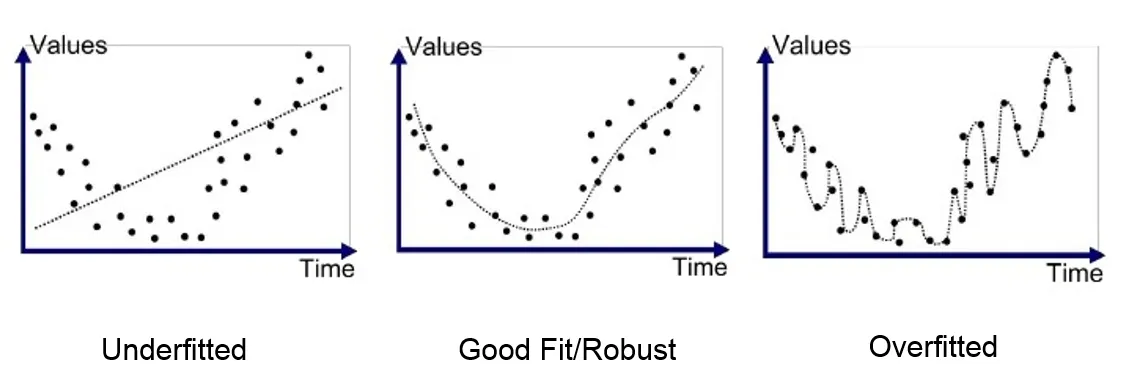
Another thing you may notice that the precision of the ELM is not as good as the Deep FFNN trained via backprop, however, some argue that this is not necessarily a bad thing. One of the criticisms of deep learning is it's tendency to overfit the training data. This is where is has become too good at learning the example data that it does not generalise to new data well anymore. (You can think of overfitting as memorising the training examples rather than learning it’s general trends)

One reason why the activation functions of neural networks are kept simple is because they need to be easily differentiable to be trainable via backprop. However, with ELMs this limitation no longer exists and so the activation functions can be as complex as you wish. Some interesting variants with more complex activation functions such as these, include kernels so that a single neuron alone can approximate more complicated decision boundaries.
A personal favourite of mine is a variant which completely remodels the neuron from scratch. The Hierarchical Temporal Memory (HTM) neuron is designed to more accurately model biological neurons (such as those in the human brain)

p.s. All code used in this blog can be run via Google Colab here: https://colab.research.google.com/github/mohammedterry/ANNs/blob/master/ANN_NeuroEvo_ELM.ipynb