Tips and Tricks for Multi-Class Classification

8 min readApr 28, 2019

Just as binary classification involves predicting if something is from one of two classes (e.g. “black” or “white”, “dead” or “alive”, etc), Multiclass problems involve classifying something into one of N classes (e.g. “red”, “white” or “blue”, etc).

Common examples include image classification (is it a cat, dog, human, etc) or handwritten digit recognition (classifying an image of a handwritten number into a digit from 0 to 9).

Intent classification (classifying the a piece of text as one of N intents) is a common use-case for multi-class classification in Natural Language Processing (NLP).

This tutorial will show you some tips and tricks to improve your multi-class classification results.

Evaluation Methods

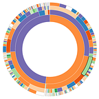
We shall have an image as our dataset to be able to qualitatively evaluate our multi-class classifiers via visual inspection. However, this is just for the clarity of the tutorial. Most real data cannot be visually interpreted so easily. Therefore we must rely on more quantitative metrics (e.g. Precision, Recall, F1, Confusion Matrix) which can evaluate the model (simpler metrics like accuracy don’t take into account unbalanced data) and see which classes the model is confusing with one another

Our target data containing 3 classes (white, red, blue)

Inherently Multi-class Classifiers

Not all models inherently support multi-class classification. Lets start by using some that do.

K-nearest-neighbours (KNN) is one of the simplest models for classification but did surprisingly well (p.s. this is not to be confused with K-means clustering).

from sklearn.neighbors import KNeighborsClassifier
knn_classifier = KNeighborsClassifier()
knn_classifier.fit(training_inputs, training_outputs)
knn_predictions = knn_classifier.predict(training_inputs)

Another model which performed well was the Random Forest algorithm (it essentially trains multiple decision-trees and averages their collective decisions together).

from sklearn.ensemble import RandomForestClassifier
rf_classifier = RandomForestClassifier()
rf_classifier.fit(training_inputs, training_outputs)
rf_predictions = rf_classifier.predict(training_inputs)

What about a feedforward Neural Network? The default shallow network (with a single hidden layer of 100 nodes) performs very poorly! It gets an f1 score of 0.8 for the white class (0) but 0.49 for the blue class (2) and even worse, 0.38, for the red class (1).

shallow feedforward neural network classifier

from sklearn.neural_network import MLPClassifier
snn_classifier = MLPClassifier()
snn_classifier.fit(training_inputs, training_outputs)
snn_predictions = snn_classifier.predict(training_inputs)

If we use a deep feedforward neural network instead (with 5 hidden layers of 100 nodes each) we get better results, with each class achieving an f1 score above 0.9. However it still isnt as good as the previous two models (achieving perfect f1 scores for each class!)

dnn_classifier = MLPClassifier(hidden_layer_sizes = [100]*5)
dnn_classifier.fit(training_inputs, training_outputs)
dnn_predictions = dnn_classifier.predict(training_inputs)

Is there something else we can do apart from adding more layers? Let’s take a look at the data!

Unbalanced Data

Our dataset is unbalanced (it has more samples for some classes than others). This can make the classifier biased toward the one or two classes with lost of samples, while dwarfing others that have less (i.e. the classifier learns the classes with more samples better and remains weak on the smaller classes).

Our dataset is unbalanced: it contains more samples for class 0 (white), than it does for class 1 (red) or class 2 (blue)

So we should balance our dataset before training our classifier. There are various methods to do this, including subsampling (taking a smaller yet equal selection of samples from each class), upsampling (taking repeat samples from some classes to increase its numbers), resampling (using an algorithm like SMOTE to augment the dataset with artificial data), etc

subsampling (left), upsampling (centre), resampling using SMOTE (right)

from imblearn.over_sampling import SMOTE
sm = SMOTE()
resampled_training_inputs, resampled_training_outputs_labels = sm.fit_resample(training_inputs, training_outputs_labels)

Ensemble of Binary Classifiers (One-vs-Rest)

Even with balanced data and a fine-tuned model, most classifiers are limited to distinguishing between a handful of classes well (they will start to struggle when the number of classes becomes very high). Therefore, if you have a lot of classes, instead of training a single classifier, you can train multiple binary classifiers (one for each class / one-vs-rest) - which is easier for each classifier to learn. Then combine each of the classifiers’ binary outputs to generate multi-class outputs.

one-vs-rest: combining multiple binary classifiers for multi-class classification

from sklearn.multiclass import OneVsRestClassifier
dnns_classifier = OneVsRestClassifier(MLPClassifier(hidden_layer_sizes = [100]*5))
dnns_classifier.fit(np.array(training_inputs), training_outputs_labels)
dnns_predictions_labels = dnns_classifier.predict(training_inputs)

Using multiple deep feedforward neural networks, we achieve slightly better f1 scores (class 0 improved from 0.97 to 0.98, class 1 improved from 0.95 to 0.97, however, class 2 reduced from 0.91 to 0.89 * this can be addressed by balancing the data).

one-vs-rest deep feedforward neural networks

Of course, this also opens up our arsenal of models (as there is a far wider range of binary classifiers than multi-class classifiers). Lets try one-vs-rest support vector machine (SVM) classifiers (an SVM creates a linear decision boundary in a higher dimensional space than the data, which translates into a non-linear decision boundary in the lower-dimensional space)

from sklearn.svm import SVC
svm_classifier = SVC(decision_function_shape='ovr')
svm_classifier.fit(training_inputs, training_outputs_labels)
svm_predictions_labels = svm_classifier.predict(training_inputs)

Or one-vs-rest xgboost classifiers (Gradient boosting is similar to a random forest in that it uses the results of many decision trees. However, in a random forest, trees are grown in parallel but are random and unrelated to each other. Each tree is grown very deep to overfit a specific part of the training data — however, in the end, all the trees’ errors cancel out when combined as different trees in the forest will overfit in different ways and thus voting averages these differences out. With boosting, however, only very shallow trees are carefully grown to find general patterns in the data. One tree is added in turn to improve / boost the already trained ensemble of trees).

from xgboost import XGBClassifier
xgb_classifier = OneVsRestClassifier(XGBClassifier())
xgb_classifier.fit(np.array(training_inputs), training_outputs_labels)
xbg_predictions_labels = xgb_classifier.predict(training_inputs)

Multi-class classification without a classifier!

An alternative approach that some people use is embedding the class label instead of training a classifier (e.g. the cluster centroid of all the vectors when clustered by class can be the vector that represents that class).

clusters = {this_class:[training_inputs[i] for i,c in enumerate(training_outputs_labels) if c == this_class] for this_class in range(n_classes)}
centroids = [np.mean(np.array(vectors), axis=0) for vectors in clusters.values()]

For example, we can embed the class labels into the same space as the training data by taking the average of the vectors for each class. This is equivalent to taking the centroid of each class’ cluster.

sentences clustered by intent. The cluster average (centroid) is taken as the class’ vector representation

Once you have a vector representation for each Class Label, a new datapoint can be compared against the class labels directly (without using a classifier) by comparing the similarity of the new datapoint’s vector and the vector for the class label ( e.g. using cosine distance). Each class is then ranked by similarity and the most similar class vector will be the predicted class for that datapoint. Et voila! (you can learn more about embedding methods in my other post: https://medium.com/@b.terryjack/nlp-everything-about-word-embeddings-9ea21f51ccfe )

from scipy.spatial.distance import cosinedef predict_class(vector, class_vectors):
  scores = [(cosine(vector, class_vector),c) for c,class_vector in enumerate(class_vectors)]
  ranked = [c for _,c in sorted(scores)]
  return ranked[0]

Unfortunately, this method is very limited. It relies on the assumption that the classes are linearly separable (i.e. each class occupies separate, distinct areas). In our particular example, each class heavily overlaps and occupies the same average space. Thus their centroids end up in approximately the same place (and each class label’s vector appear very similar!)

The centroid of each class is almost the same in our example, so the class vectors will be very similar. Class 0 (white) on the left, class 1 (red) in the middle and class 2 (blue) on the right

poor classification results for non-linearly separable data (left: intended classes, right: predicted classes without a classifier)

So even though the simplicity of the no-classifier solution is attractive, it actually equates to using a very simple multi-class classifier with linear decision boundaries. If you have non-linearly separable data (as with our example), then even using a basic classifier like knn would yield better results.