For solar power to be used effectively, irradiation forecasting technology is essential. With a vast amount of data in a centralized manner, current irradiation forecasting techniques have demonstrated exceptional performance. However, current forecasting approaches are challenged by privacy protection and data security problems that may surface during the data collection and transmission process from spread points to the centralized server. In this article, a federated learning (FL) and deep learning (DL)-based solar irradiation forecasting technique is proposed.
What is Federated Learning?
A decentralized machine learning method called federated learning involves multiple clients—that is, devices or organizations—collaborating to train a model while maintaining local copies of their data. Each client trains the model using its local data; rather than sending raw data to a central server, it only sends model changes (such as gradients or weights) to the central server, which then combines these updates to enhance the global model. As a result of the raw data never leaving the clients’ devices, this method improves data security and privacy.
Federated Learning Implementation?
A fleet of Photovoltaic (PV) systems, each representing a client, can collaborate to create a data-driven model for predicting solar irradiance without sharing operational data. The FL training process is iterative, involving clients sending their model parameters to a server. The server aggregates these weights, resulting in a global FL model for all PV systems, including solar irradiance forecast information from other clients. The following paragraph contains a detailed explanation with diagrams.
Dataset:
The four months of meteorological data (September through December 2016) in the dataset are from the HI-SEAS weather station.
The dataset includes several features, such as
- Solar Irradiance[W/m²]
- Temperature [F]
- Pressure in the atmosphere [Hg]
- Humidity [%]
- Wind speed [Miles/h]
- Direction of the wind [degrees]
The following URL will allow you to get the dataset:
https://www.kaggle.com/code/enricobaldasso/prediction-of-solar-radiation-data/input
Federated learning involves the following iterative steps:
- Server Initialization:
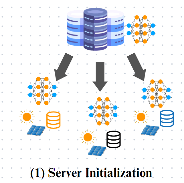
- The process starts with a central server. A machine learning model (typically a neural network) that will be utilized for classification or prediction tasks is initialized by this service.
- To capture general patterns, the model is usually pre-trained on a limited dataset (such as historical solar energy data).
2. Client Update (Local Training):
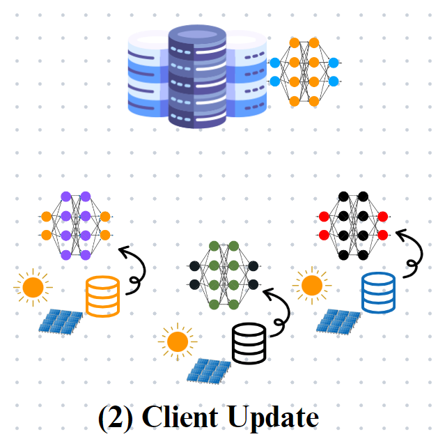
- Next, the server distributes this initial model to various local devices or clients. These clients represent individual data sources, such as solar panels installed in different locations.
- Each client performs local training using its own data.
- During local training, the model parameters are updated based on the client’s data. Gradient descent or other optimization algorithms are commonly used for this purpose.
- Importantly, raw data remains on the local device, ensuring privacy. Only model updates (gradients) are shared with the server.
3. Server Aggregation (Global Model Update):
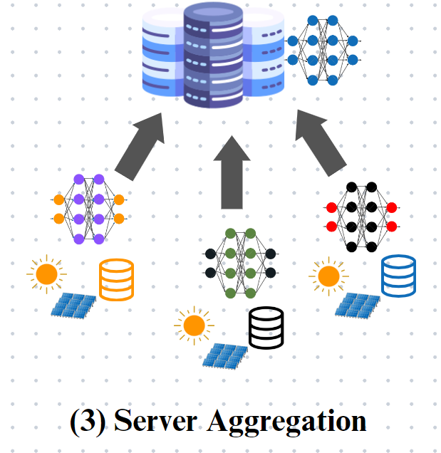
- The server compiles client updates to produce a global model after receiving them. Federated Averaging is one technique that can be used for this aggregate.
- The global model benefits from insights obtained across all clients while protecting data privacy. As more clients participate over time, the accuracy increases.
4. Server Broadcast (Model Deployment):
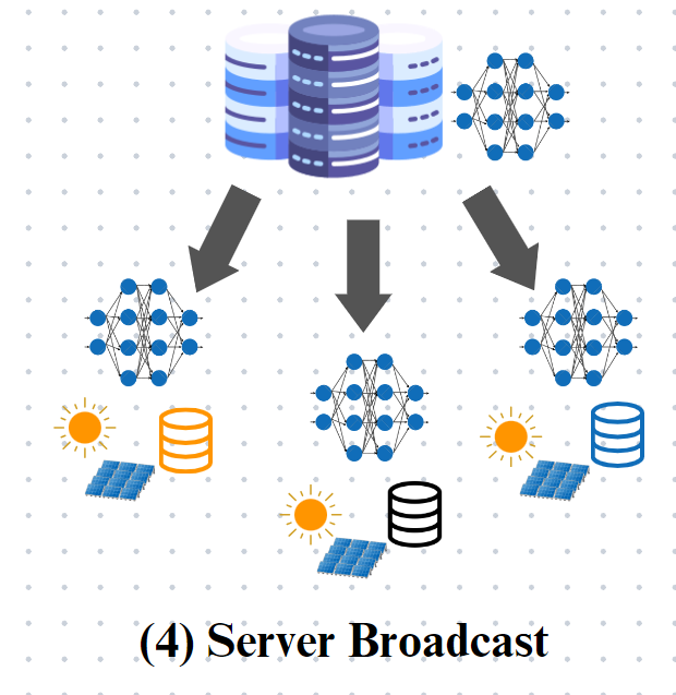
- Finally, the server broadcasts the updated global model back to all clients.
- Each client replaces its local model with the new global model. This ensures that all nodes benefit from collective knowledge without sharing raw data.
- The process repeats iteratively: local training, aggregation, and model deployment, allowing the model to adapt to changing conditions.
Data Preprocessing:
This includes
Data Cleaning: data is free from duplicates, missing values, and outliers.
Data transformation: converting data into the desired form.
Data normalization: scaling numerical data into a standard range.
Data Division:
We split the dataset into 4 clients since we are using FL on a single dataset. c1, c2, c3, and c4 are 4 clients.
#spliting the data into train and test data
xtrain, xtest, ytrain, ytest = train_test_split(X, Y, test_size=0.2, random_state=42)

c1_x=xtrain.iloc[0:7000]
c1_y=ytrain.iloc[0:7000]

c2_x=xtrain.iloc[7000:14000]
c2_y=ytrain.iloc[7000:14000]

c3_x=xtrain.iloc[14000:21000]
c3_y=ytrain.iloc[14000:21000]

c4_x=xtrain.iloc[21000:]
c4_y=ytrain.iloc[21000:]
Model Initialization:
def create_model():
    model = None
    model = Sequential()

    model.add(Dense(128, activation='relu', input_dim=14))
    model.add(Dropout(0.33))

    model.add(Dense(64, activation='relu'))
    model.add(Dropout(0.33))

    model.add(Dense(32, activation='relu'))
    model.add(Dropout(0.33))

    model.add(Dense(1, activation='linear'))

    return model
The create_model function creates a neural network with two hidden layers (64 and 32 neurons, respectively) and an input layer (128 neurons), all of which use Dropout and ReLU activation for regularization. The last layer has a single neuron with a linear activation function that forecasts solar irradiation.
FL model training & evaluation:
#model training & evaluation
model_server=create_model()
model_server.compile(metrics=['mse'], loss='mae', optimizer=Adam(learning_rate=0.001))

model_c1=create_model()
model_c1.compile(metrics=['mse'], loss='mae', optimizer=Adam(learning_rate=0.001))

model_c2=create_model()
model_c2.compile(metrics=['mse'], loss='mae', optimizer=Adam(learning_rate=0.001))

model_c3=create_model()
model_c3.compile(metrics=['mse'], loss='mae', optimizer=Adam(learning_rate=0.001))

model_c4=create_model()
model_c4.compile(metrics=['mse'], loss='mae', optimizer=Adam(learning_rate=0.001))

mae_list=[]

rounds=40
for i in range(rounds):
    print('')
    print('round-{}'.format(i+1))
    #client-1 model
    model_c1.set_weights(model_server.get_weights())#model updation
    model_c1.fit(c1_x,c1_y,validation_split=0.1, epochs=1, batch_size=32)#model training

    print('*********************************')
    #clinet-2 model
    model_c2.set_weights(model_server.get_weights())#model updation
    model_c2.fit(c2_x,c2_y,validation_split=0.1, epochs=1, batch_size=32)#model training

    print('***********************************')
    #client-3 model
    model_c3.set_weights(model_server.get_weights())#model updation
    model_c3.fit(c3_x,c3_y,validation_split=0.1, epochs=1, batch_size=32)#model training

    print('***********************************')
    #client-4 model
    model_c4.set_weights(model_server.get_weights())#model updation
    model_c4.fit(c4_x,c4_y,validation_split=0.1, epochs=1, batch_size=32)#model training

    #model aggregation and averaging

    avg_weights=[(model_c1.get_weights()[i]+model_c2.get_weights()[i]+model_c3.get_weights()[i]+model_c4.get_weights()[i]+model_server.get_weights()[i])/5 for i in range(len(model_server.get_weights()))]

    #server model updation
    model_server.set_weights(avg_weights)

    mae = mean_absolute_error(ytest,model_server.predict(xtest))

    mae_list.append(mae)

    print(f'mean absolute error: {mae}')
For each round, the following steps are repeated:
- Model Update for Clients: Each client model updates its weights to match the current server model (
model_server.get_weights()). - Model Training for Clients: Each client model is trained on its local data (
c_x, c_y) for one epoch.
DL model training & evaluation:
model = None
model = Sequential()

model.add(Dense(128, activation='relu', input_dim=14))
model.add(Dropout(0.33))

model.add(Dense(64, activation='relu'))
model.add(Dropout(0.33))

model.add(Dense(32, activation='relu'))
model.add(Dropout(0.33))

model.add(Dense(1, activation='linear'))

model.compile(metrics=['mse'], loss='mae', optimizer=Adam(learning_rate=0.001))

history = model.fit(xtrain, ytrain, validation_split=0.1, epochs=40, batch_size=32)
comparison of models (FL vs Non-FL):
fit=history.history
plt.title('mean absolute error(mae) vs epochs of mlp')
plt.xlabel('epochs')
plt.ylabel('mae')
plt.xticks(range(0,len(mae_list),2))
plt.plot(mae_list,marker='*',label='FL',color='blue')
plt.plot(fit['loss'],marker='+',label='NoFL',color='red')
plt.legend()
plt.show()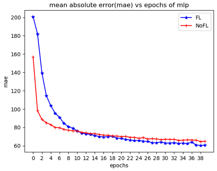
The blue line represents the MAE for the federated learning (FL) setup, while the red line represents the MAE for the non-federated learning (Non-FL) setup.
Key Observations:
- The FL model starts with a higher MAE, suggesting that FL may initially be slower in reducing errors compared to the Non-FL approach.
- Both FL and Non-FL configurations exhibit a declining trend in MAE as the epochs increase, suggesting that the models are learning and enhancing.
- After about 20 epochs, the Non-FL approach is slightly outperformed by the FL approach, indicating that the FL approach can provide both accuracy and data privacy, albeit with a slower convergence speed.
For accessing python notebook, please visit:
Remarks:
Federated learning essentially opens the door to a future in which intelligent systems might gain from shared information without compromising personal privacy. The use of FL in solar irradiance prediction is only one example of how this technology may propel advancement in a variety of fields, enabling a more linked and safe society. As we progress, the principles and results of federated learning will definitely inspire and define the next generation of AI applications.
Real-World Example: Google’s Gboard uses FL to improve typing predictions and suggestions across millions of devices while maintaining user privacy.
Acknowledgements and References
This federated learning project was guided and supported by Dr. (Mrs.) B. Janet of the National Institute of Technology, Tiruchirappalli (NITT).
