Reinforcement Learning: An introduction (Part 2/4)

Welcome back to part 2 of the intro to reinforcement learning series!

In part 1 we described what reinforcement learning (RL) is, what you can do with it and some of the challenges of RL. This time around, we will explain some of the main concepts of RL and introduce some terminology and notation. This will be useful for the next part, where we discuss a simple RL algorithm.

Specifically we will talk about:

• States
• Actions
• Reward functions
• Environment dynamics (Markov Decision Processes)
• Policies
• Trajectories and return
• Value function & Q-function

As always, if you’re already familiar with the content, feel free to head on to the next part.

Note: If you are reading this on a smartphone browser, you might not be able to view the subscripts. You can download the Medium app to mitigate this.

The RL framework

Let’s start with a quick recap. The RL framework involves an agent that tries to solve a task in a certain environment. At every timestep t, the agent needs to choose an action a. After this action it might receive a reward r and we get a new observation of its state s. The new state can be determined both by the action of the agent and also by the environment the agent is operating in. In RL we want to maximize the future accumulated reward.

For the sake of explanation, we will use the game of Pong to further explain these concepts.

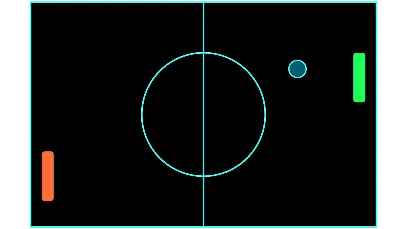
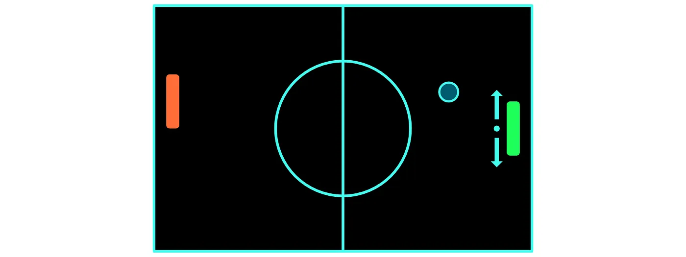
Pong is an easy game to explain: There are two players, represented by the green and the red paddles in the image above. In our example, we will consider the player who operates the green paddle to be our agent. The goal of Pong is to bounce back the ball, past the other players’ paddle. When either player manages to bounce the ball past the other player, they get a point and the ball starts moving from the centre of the field again. The player with the highest score wins.

Here is a 1 hour long gameplay video if you are still confused.

How do the different terms of the RL framework apply when we want to train an RL agent to play Pong?

States

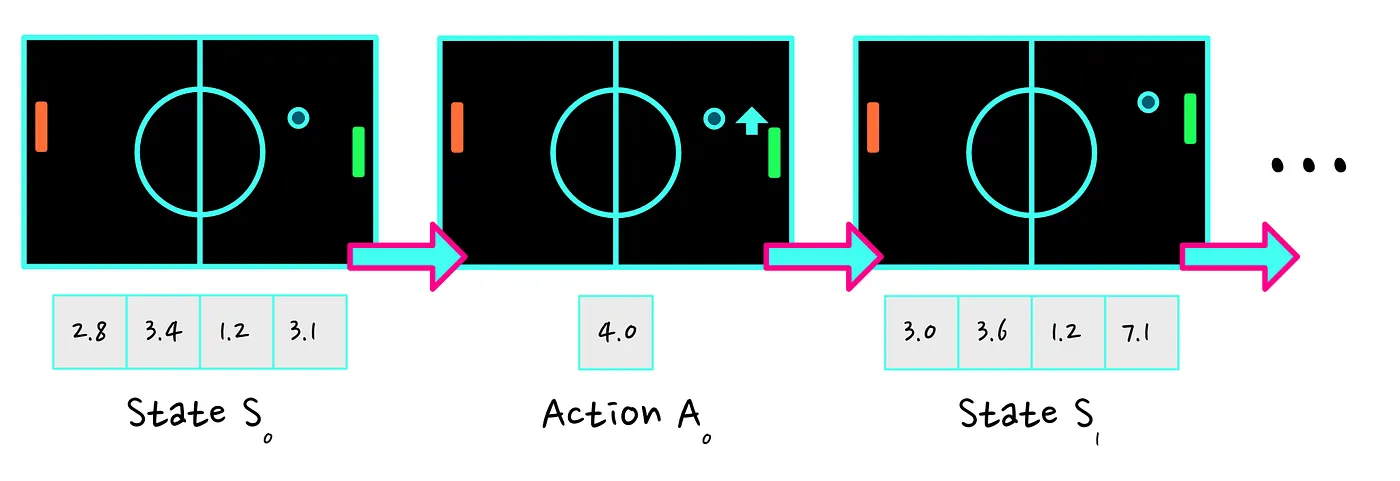
Let’s start with the state. A state is usually a vector, matrix or other tensor. If you are not familiar with these terms, don’t worry, they are essentially various ways of organising numbers. You can check the image below as an example.

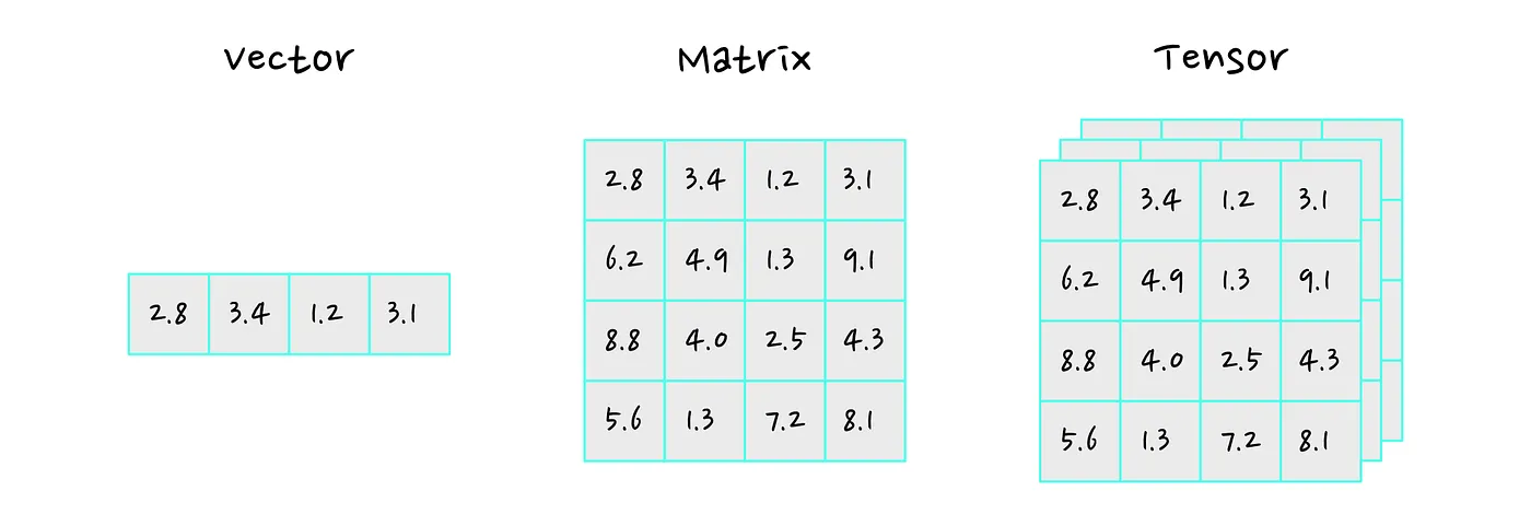
The state should describe the relevant information we need in order to decide which action to take at timestep t. We will denote the state at timestep t as sₜ .

In the case of Pong, a good description of the state can be a vector (an array of numbers) containing the position of the players’ paddle, the position of the ball and the angular velocities of the ball. This would be enough for our agent to decide whether it’s best to move the paddle up or down. Because from this information it can check its own position, the position of the ball and where the ball is moving towards.

Note that it wouldn’t suffice to only encode the position of the ball and the player, because we also need some information that indicates in which direction the ball is moving.

Another option would be to directly use the frames/pixels of the game to represent the state. The state is then a matrix or tensor representing the light intensities/colours of the pixels. This will be harder for the AI algorithm to learn, but it is definitely possible. It will be harder, because now it not only needs to learn how to play the game, but it also needs to learn how to extract the relevant information from these pixels. It will need to learn that for example the blue pixels in the middle represent a ball and it will need to learn that the location of this ball is relevant in solving this problem.

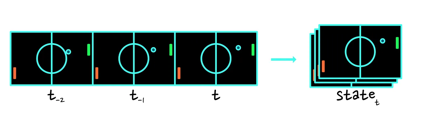
Note: We also encounter the same problem as the one we encountered when we used a state vector, namely: one static image is not enough to show in which direction the ball is moving. As a solution, the state is often represented as a stack of the last few frames.

As a final remark, even though we are using the term “state”, the term “observation” is more appropriate. The difference is that a state is assumed to give a full description of the state of the world, while the term observation refers to a (possibly partial) observation of the state. For our purposes, we will use these terms interchangeably.

Actions

In Pong we want our agent to be able to move the paddle up and down.

There are various ways of representing this action, but first there is an important distinction to make about actions in RL in general. We will make a distinction between discrete action spaces and continuous action spaces.

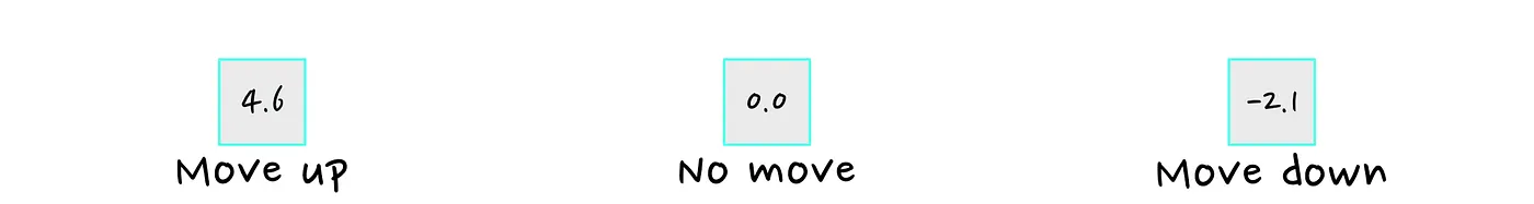
In the case of a discrete action space, our actions are discrete, this means that they can take on only a certain set of values. For example in the game of Pong, we could define our actions to be “Up”, “Down” and “No move”. This means that our paddle can move up, down or stand still at every timestep, but only by a predefined amount. Moving up could mean that we move up by 10 pixels every time for example.

To represent these three actions, we could use a vector (row of numbers), where each dimension (column) of the vector indicates which action to take. Normally the values in the vector are still continuous and represent “a categorical distribution” of which action the agent should take. You can disregard this for now and just look at this as “the dimension in the vector where the number is 1, is the action our agent will take”.

In the case of a continuous action space, our actions are continuous, meaning that they can take on any value. So if we look at the game Pong, now our action might not just represent the paddle moving up our down, but we might also specify by how much the paddle should move up or down. In this case, a vector with a single dimension (a scalar) will suffice. The scalar can have a positive value for moving up, 0 for not moving and a negative value for moving down.

Reward function

The reward function tells us after every action how much reward the agent got for taking that action. Or more precise: the reward function takes a state Sₜ and an action Aₜ as input at every timestep t, and outputs a reward Rₜ . The reward Rₜ is a scalar (number) that indicates how well the agent did.

In Pong, we could opt for giving a reward of 1 every time the agent manages to make the ball go past the other players’ paddle, 0 when nobody scores, and -1 when he misses the ball causing the opponent to score.

Formally, the reward function has the following signature:

Where S represents the set of states, A the set of actions and ℝ the set of real numbers.

You should be careful when choosing how you define the reward the agent receives, as this can highly affect its behaviour. For example, it can produce unforeseen consequences or if your agent sees too little rewards (sparse reward problem), it might fail to learn anything at all.

Environment dynamics

The environment dynamics answer the following question: given a state and an action, what will be the next state? Typically, we don’t need to model these environment dynamics ourselves. Our RL algorithm will need to figure them out on its own. Even more so, for many problems the environment dynamics are unknown.

We will briefly talk about the idea of environment dynamics nonetheless, because the only requirement for us to be able to apply RL to a problem, is that we are in theory able to define the problem as a Markov Decision Process (MDP).

A Markov-what you ask? You will see this term come up in a lot of the literature around RL and the reason for this is that MDP’s are a way of formalising problem statements. They will also help us explain some of the algorithms we will use later on. Let’s talk about MDP’s for a moment.

Markov Decision Process

An MDP is a discrete-time stochastic control process that has the Markov property. This is a mouth-full, but it’s not so complicated. Let’s break it down.

We are describing a process in which we have a set of states. These are the states that our agent can be in during the process of solving a problem. The process is modelled in discrete time, which roughly means that everything that happens is represented as a separate point in time. In other words, you cannot be “in between” two states, either you are in a state or you are not. A point in time is then represented by a number and the next point in time would be that number +1.

We also define a transition distribution:

A transition means we are going from one state to another. So this formula tells us the probability of going to a next state sₜ₊₁, given our current state sₜ and taking an action aₜ. That is the “stochastic” part of our definition, stochastic simply means that we are dealing with probabilities. So sometimes our agent might decide to take an action, but because of the environment, there might not be a guarantee that he ends up in the state the agent intended.

Last but not least, our control process needs to have the Markov property. Markov refers to its inventor, Andrej Markov. The property tells us that any next state only depends on the current state. When a process has the Markov property, the next state does not depend on any other states except for the current one. So our agent might have seen a million states before, but still it won’t matter to determine the next state, only the current state does.

The diagram below shows an example of such a process. The circles containing S₀-S₂ represent states, while the pink circles represent actions that can be taken in those states. S₀ is green, because it represents a starting state. Most processes also have terminal states (states that mark the end of the process), but they are not drawn here.

If you are in state S₂ at timestep t for example, you can take actions A₀ or A₁. If you opt for action A₀, then you have a 26% chance of ending up in state S₀ at time t+1, while you have a 74% chance of ending back up in state S₂ at t+1. Notice that it doesn’t matter which states we have previously visited to determine our next state.

Great, that’s all there’s to it, now you know what an MDP is! Now what would an MDP look like for the game Pong? We have already discussed what the states and actions of our agent can be. The states describe the positions of the paddles and the ball, as well as the speed of the ball. The actions we can take are move up or down.

In the case of Pong we are dealing with an environment that is fully observed, we have access to all information in this game. This is not always true, sometimes our environment can only be partially observed. Think for example of a game of cards, where you cannot see the cards your opponent is holding.

Our environment, as we currently described it, is still stochastic however. The reason for this is mostly due to our opponent. Say that our paddle is at position X1 while our opponent is at position X2. Even though we decide how our paddle will move and the physics of the moving ball might be deterministic, our opponents’ paddle might move randomly or probabilistically.

Policies

Alright, we have a lot of terms to cover in today’s post, next up are policies. When we talk about a policy, we are referring to the “behaviour” of our agent. Given a state, what should be the next action the agent takes? This is the crux of our algorithm.

Similar to what we did for actions, we will distinguish between deterministic policies and stochastic policies. We can write a deterministic policy as:

In this formula, aₜ is an action at timestep t, sₜ is the state at timestep t, and μ is our policy function with parameters θ. You can simply look at this formula as a mathematical function that receives some input (the state) and then outputs a corresponding action for the agent to take. The parameters θ influence the output of the function, so we want to change these such that our agent behaves in a way that optimally solves the problem. We will see in the next blog post how we do that, don’t worry about them for now.

A stochastic policy on the other hand, would look like this:

This formula is very similar to the deterministic policy. aₜ is an action at timestep t, sₜ is the state at timestep t, and π is our policy function with parameters θ. It is a convention to use π for stochastic policies. The difference with the deterministic policy, is that we select action aₜ with a certain probability, but it could very well be the case that the next time we are in a similar state, we select a different action instead.

Neural networks

You might wonder, these policies look nice, but what function do we use to model them?

In practice, we will often use a neural network (NN)for these functions. Remember, we are trying to create a self-learning system after all. We will very briefly explain what a neural network is and how it works.

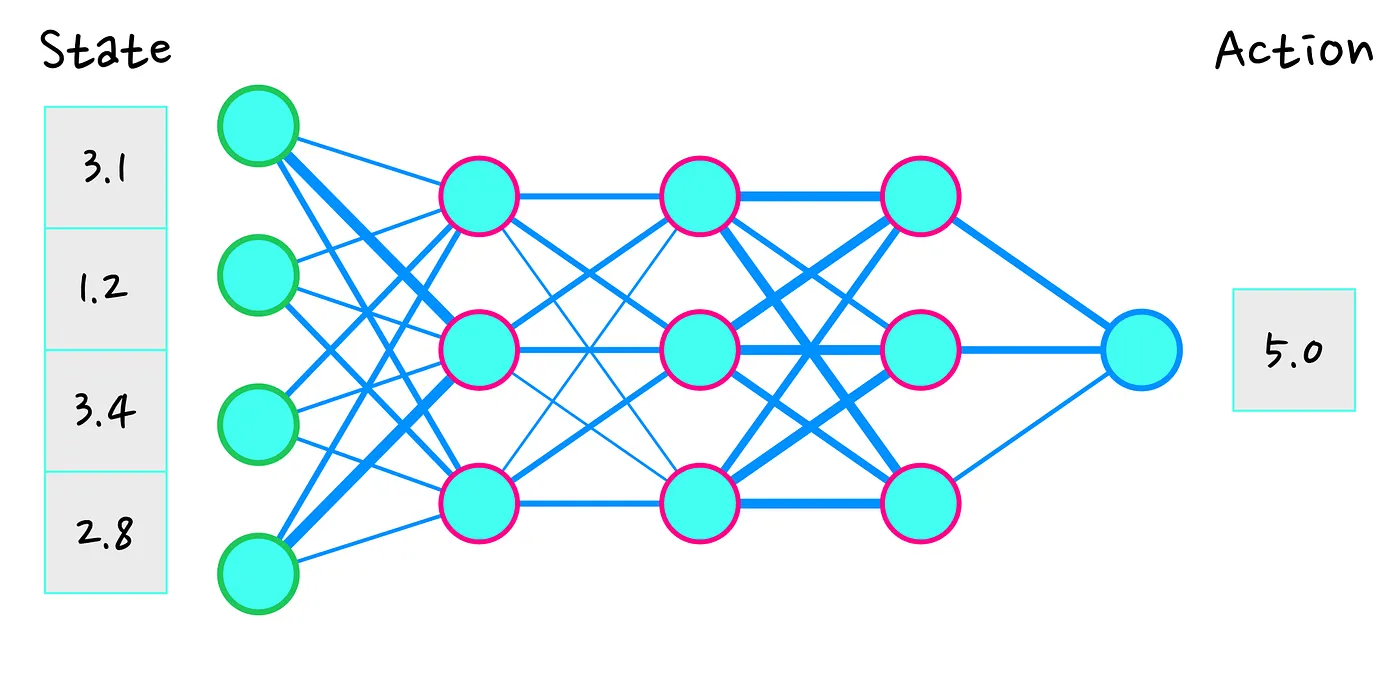
A neural network (NN) is a learning structure loosely based on the human brain. It consists of neurons (the cyan dots in the picture) and synapses (the blue wires between the blue dots). When you look at the NN, you can see that it has various “columns” of blue dots, we will call those layers. The first layer (blue dots with green edge) we call the “input layer”. The final layer (a single neuron with blue edge) we call the output layer.

A NN works by taking some numbers as input, starting at the -you guessed it- input layer. This input is similar to an electrical signal arriving at the brain, and passing through it. The synapses (connections) reinforce or weaken the signal. Then, the signal from various neurons gets combined, right before it arrives at a new neuron in the next layer. If the signal is strong enough, the neuron will “fire” and propagate the signal further, if it is not strong enough, it will not propagate the signal. This process continues, until the signal arrives at the output layer and thus gives us an output. So in our case, the state will be the input to the network, and the number (or numbers) it outputs will be the action of our agent.

Initially the NN is wired randomly, so the signal will also be strengthened and weakened randomly, and thus produce a random output/action. The trick is now for us to change the connections in such a way that the neural network produces an output that is closer to the one we were expecting. You can look at the NN as a big machine with a lot of knobs, and now we need to figure out how to turn the knobs until it produces satisfactory output. We can do this using mathematics, through an algorithm called backpropagation. But we will omit details for now.

Remember the parameters we were referring to when talking about policies? In the case of a neural network, they are in fact referring to these connections! Changing the connections is our way of changing the output the policy produces.

We have covered a lot of ground already and we are nearly ready to complete this article full of definitions and notations. I promise you, they will all be useful later on when we get to the actual coding of these algorithms!

Trajectories and returns

Trajectories are easy to understand once you know about states and actions. A trajectory is simply referring to a certain sequence of states and actions:

At the end of a trajectory, our agent will have accumulated a certain amount of rewards. This accumulated reward is what we call the return.

We distinguish between finite-horizon and infinite-horizon returns. A finite horizon means that our trajectory will consist only of a limited amount of timesteps, while an infinite-horizon means we will calculate the return for infinite timesteps.

This is the formula for the finite-horizon return. We have a trajectory τ for which we calculate the return R(τ). In the formula, we take the sum of every rₜ for timestep 0 until horizon T.

The formula for the infinite-horizon return is quite similar, except we are now summing over a theoretical infinite number of timesteps and we introduced a new variable γ. The γ (gamma) is the discount factor, its value is always between 0 and 1 (inclusive). The lower the discount factor, the less valuable future rewards will be.

The discount factor is both mathematically convenient and it has an intuitive interpretation as well. It is convenient because for problems with infinite timesteps, we know that it will converge to a finite value. On the other hand, it is also intuitive to think that it’s usually better to get rewards rather sooner than later. It is for example better to get cash now than later, because due to inflation the cash might be worth less later.

Value function and Q-function

In RL we are looking to find a policy (a behaviour) for our agent such that it will receive the highest possible cumulative reward. In order to discover this policy, there are some other useful functions we can define, like the Value function. The value function looks like this:

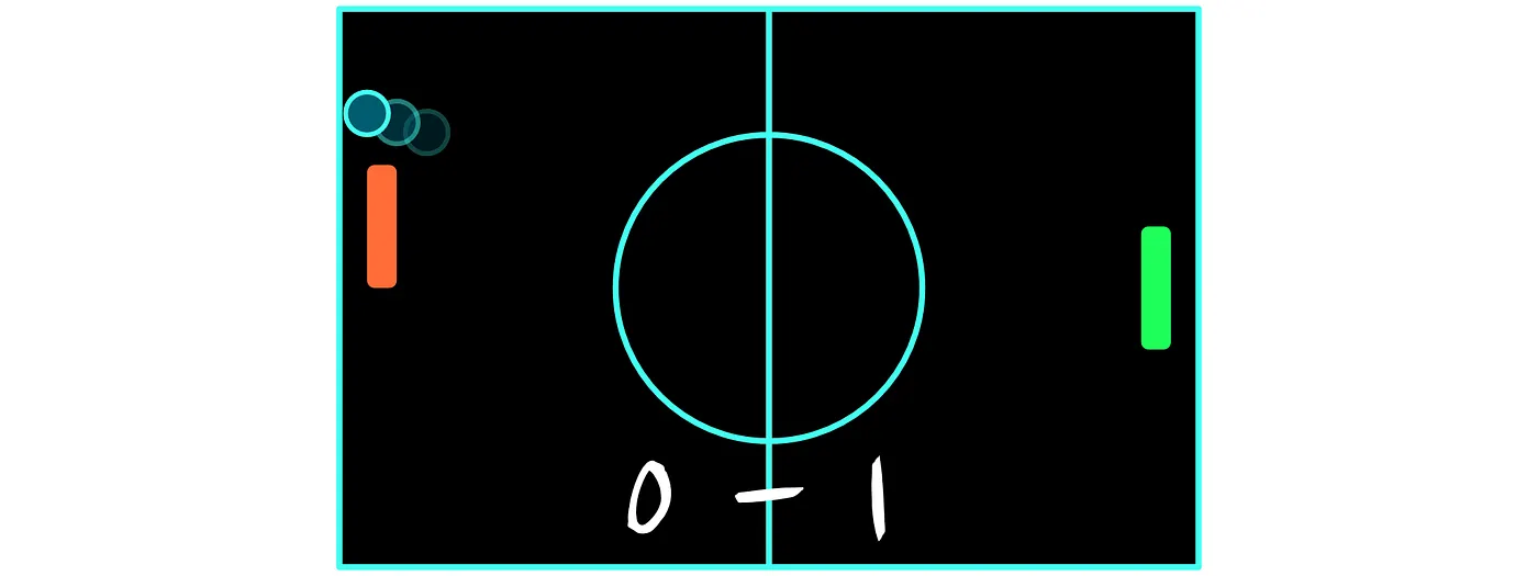
You can read this formula as: “The value of being in state s, while acting under policy π, is equal to the reward we get of the trajectory τ that we expect to follow from policy π, given that state s is the starting state.” Or in short, it roughly tells us how good it is to be in a certain state. The “E”-symbol in this formula stands for “expectation”. It is the trajectory we expect to get from policy π, the average trajectory if you will.

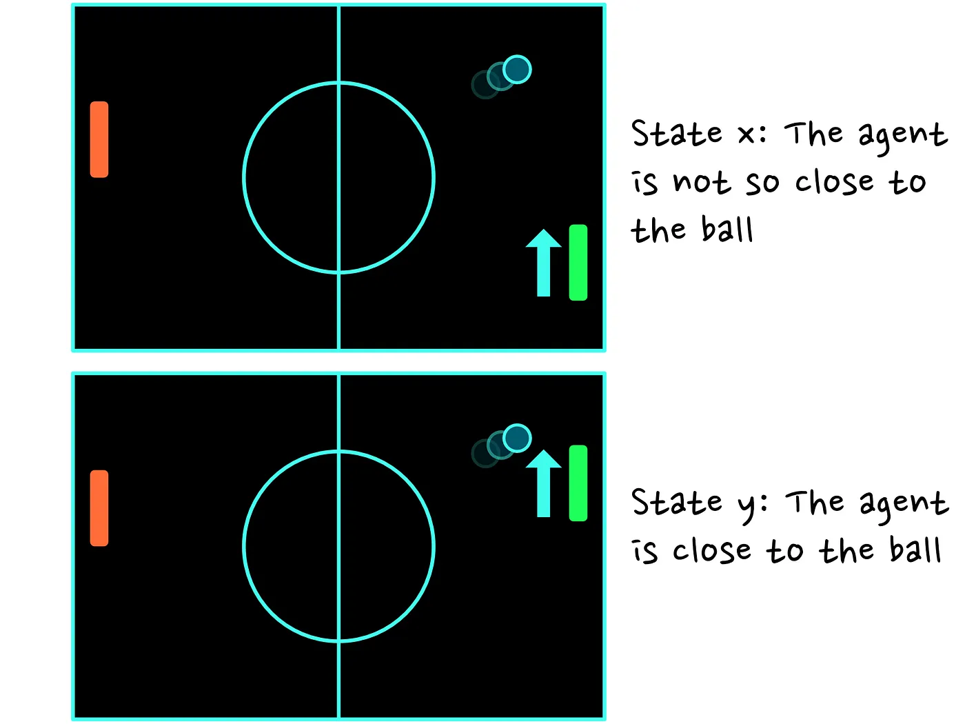
As an example, have a look at the above image. In the top image, our agent is very far from the ball, while in the bottom image, our agent is pretty close to the ball. If our agent has a policy that makes him move towards the ball, then it is highly likely that the value of state Y is higher than the value of state X. The reason is that in state X, our agent might not be able to make it to the ball in time, thus losing him the point.

Another function that turns out to be very useful is the Q-function. It looks like this:

As you can tell, it looks rather similar to the value function, and it is in fact similar, with one subtle difference. The function says :“The value of being in state s and taking action a, while acting under policy π, is equal to the reward we get of the trajectory τ that we expect to follow from policy π, given that state s is the starting state and the first action we take is a.” Or in short, it tells us how good is it to be in a state and to take a certain action.

Both of these functions are often used in RL algorithms. They have whole families of algorithms associated with them. For example, Q-learning algorithms are based on exploiting the fact that if you know the Q-value for all possible actions in a state, then you can decide which action is best to take. You will get an optimal policy simply by picking the action that has the highest value for the Q-function.

Unfortunately, in most cases we can’t know the Value function or Q-function exactly, so in practice we will estimate/learn them using learning algorithms (like a neural network).

Conclusion

This was a long post full of terminology, but you made it! Having talked about all these concepts, will give you a solid basis to start implementing your own algorithm. In the next part we will talk about the REINFORCE algorithm. The REINFORCE algorithm is conceptually simple, but lies at the heart of the policy gradient-family of algorithms. Thank you for reading and see you in the next part!