Reinforcement Learning: An introduction (Part 4/4)
Welcome back to the final part of this introduction series to Reinforcement Learning!
In this final part, we are going to make our hands dirty and implement the REINFORCE algorithm that we talked about in part 3. After this you will have a working algorithm that you can use to solve some simple tasks. On top of that, you should have a proper understanding of Policy Gradient algorithms, which you can use to tackle more complex problems and algorithms.
The content of today looks like this:
- Development Environment Setup
- The RL Environment Abstraction
- Implementing REINFORCE
- Conclusion
Let’s dive in!
Development Environment Setup
The first thing every developer needs is a development environment. I don’t want to enforce any specific setup or tools, but in case you are a beginner, I will just walk you through to the tools I personally use.
IDE (Code editor)
My choice of code editor is Visual Studio Code. It is a lightweight editor which you can use for multiple programming languages. The editor comes out of the box with very minimal tooling, but allows you to add more functionality through extensions.

Python
The programming language we will be using is Python, a high-level programming language. By high-level we mean that the language takes care of a lot of things for you like memory management. It is also an interpreted and dynamically typed language. You can simply download and install Python like any other application. Personally I use version 3.8 for maximum compatibility with several libraries, but for this tutorial you can just go on and install the latest available version.
Virtual environment setup (Optional, recommended)
For this tutorial we will be using some libraries (code that we import to use in our own project). You typically install these libraries through a package manager. In the case of Python, the default package manager is called pip. We will use pip to install some packages. It is however a good idea to create a so-called virtual environment. A virtual environment isolates the packages you installed from other (virtual) environments. Having this isolation is often a good idea, because it allows you to install multiple versions of a package at the same time (but in different environments).
There are multiple benefits of creating a virtual environment and also multiple ways to do it. For now we will just look at one particular way. We start by opening a terminal. Navigate to the folder where you intend the code to be and type the following commands:
# For Windows
py -m venv env# For Mac OS/Linux
python3 -m venv env
This tells Python (version 3.X) to create a new virtual environment named env. Next up, we will need to activate this environment by using:
# For Windows
\env\Scripts\activate# For Mac OS/Linux
source env/bin/activate
That’s it! Commands you enter will from now on be executed in your virtual environment. To deactivate the environment, simply type deactivate. To activate the environment again, simply type the command mentioned above. Do make sure you are in the same folder as where you have created the environment (your project folder).
PyTorch
In the next step of our setup, we will install a deep learning framework. There are many frameworks available, but the industry standards at the time of writing are either TensorFlow or PyTorch. We will be using the latter one although nothing prevents you from opting for TensorFlow (or other frameworks) instead.

In previous posts we talked about neural networks, gradients etc. PyTorch will make abstractions of a lot of these things for us and make our life easier by providing ready to use implementations for these concepts.
In order to install PyTorch, you will need to open a terminal and enter the commands provided to you on this website:
https://pytorch.org/get-started/locally/
You should select Stable, your operating system, Pip, Python and Default.
Additional packages
Some smaller additional pip packages we will use are:
You can just use “pip install nameofpackage” to install these.
The RL Environment Abstraction
In order to train our RL algorithm to solve “any” problem, we are going to make an abstraction of the environment. For this we will use the popular framework called Gym by OpenAI:
You can install the Gym framework like any other pip package from the link above. Crucially, Gym provides us with several abstractions that we can apply to any environment and problem:
- You can create an environment with gym.make(“environment-name”) function
- After creating the environment, you can use the env.step(action) to take an action and go to the next state. This function will provide you with the observation of the next state, the reward granted, a boolean indicating whether the episode ended, and some optional metadata
- The env.reset() function will reset the environment to a starting state (and return the values of this starting state)
- Finally, the env.close() function will clean up any resources allocated by the environment
We will go even one step further than using vanilla Gym. We will write our own Environment class, which contains some additional variables and helper functions, which will mostly help us later on when implementing more complex algorithms.
Implementing Reinforce
We will now start writing some code. First we will need a class that can represent our policy (Neural network).
Neural Network
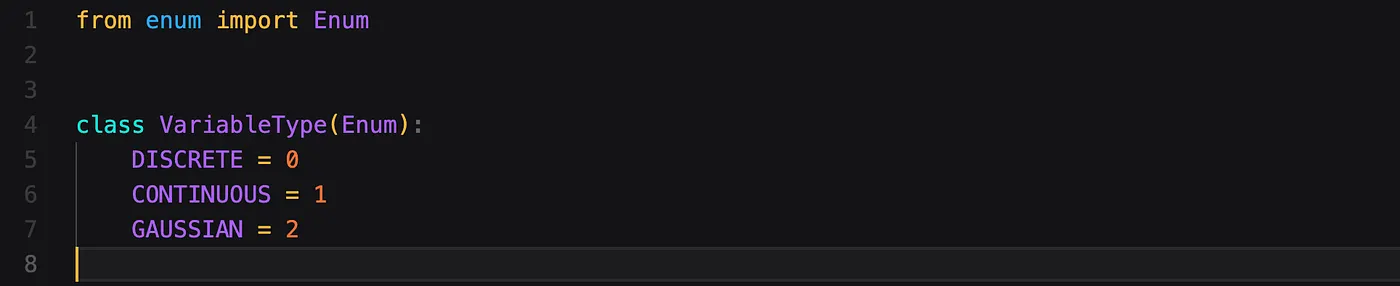
We start by defining a small enumeration. We will use this Enum to distinguish between the different types neural networks we could expect.
- Discrete represents a discrete output, or more precisely a distribution of probabilities over a fixed number of dimensions.
- Continuous represents a continuous value.
- Gaussian represents a gaussian distribution output, meaning we output a mean and standard deviation.
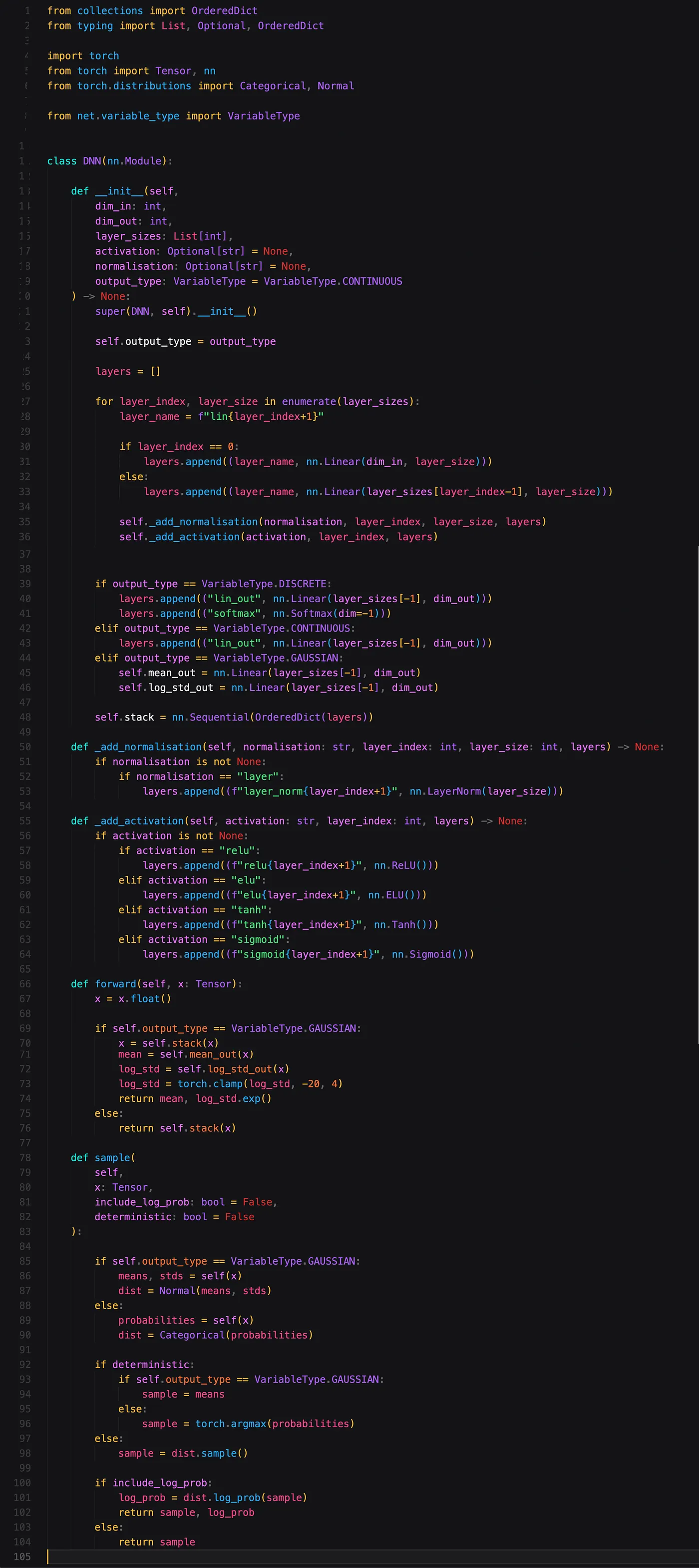
Our next class represents our neural network. We start with a fairly complex constructor (the __init__ function). Even though there is a lot of code, all this constructor does is construct a neural network, given some configuration. The most crucial parameters are dim_in, dim_out and layer_sizes. They represent the input dimension size, output dimension size and the number of neurons in the hidden layers, respectfully.
Next we have a forward function, which is typical in PyTorch. This function does a forward pass through our neural network (see the resources here if you want to learn more about how PyTorch handles neural networks).
Lastly we have a sample function. This function performs a forward pass through the network, constructs a distribution (categorical or gaussian) and then takes a sample from it. Optionally you can pass a boolean called deterministic, in which case either the mean of the gaussian will be returned, or the index of the dimension where the categorical distribution is highest.
Environment
As mentioned earlier, we will also create our own abstraction of an environment, on top of the Gym abstraction. We do this to make experimentation a bit easier and such that we have to write less code to try out a different environment. Later on this abstraction will also help us with implementing some more complicated algorithms that require us to overwrite some functions (for example in case we need a custom reward function).
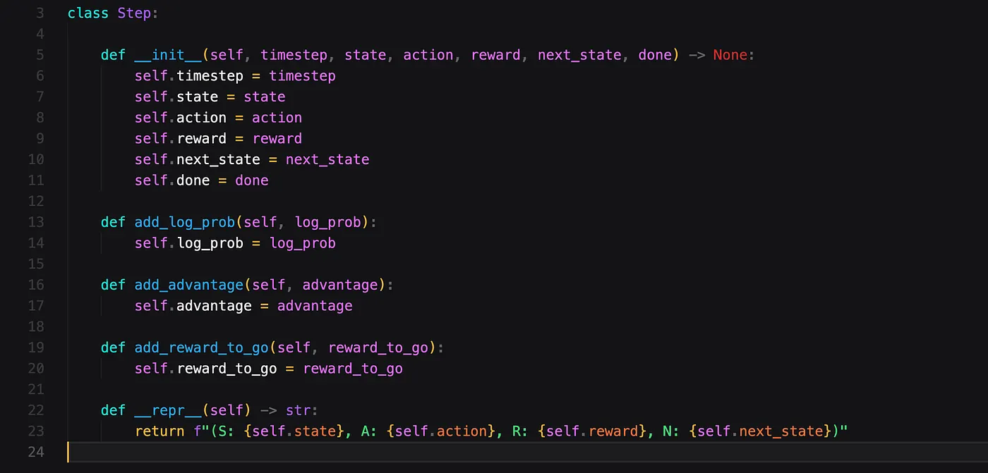
We start with a simple Step class, which represents a step in the environment. Essentially the Step class is just a data container class.

Our Trajectory class holds an array of Steps. Besides this, it contains some helper functions to convert the values these steps contain to Tensors. A Tensor is a data object from PyTorch which will make our computations more efficient. It also contains a helper function to compute the score of a trajectory and the length.
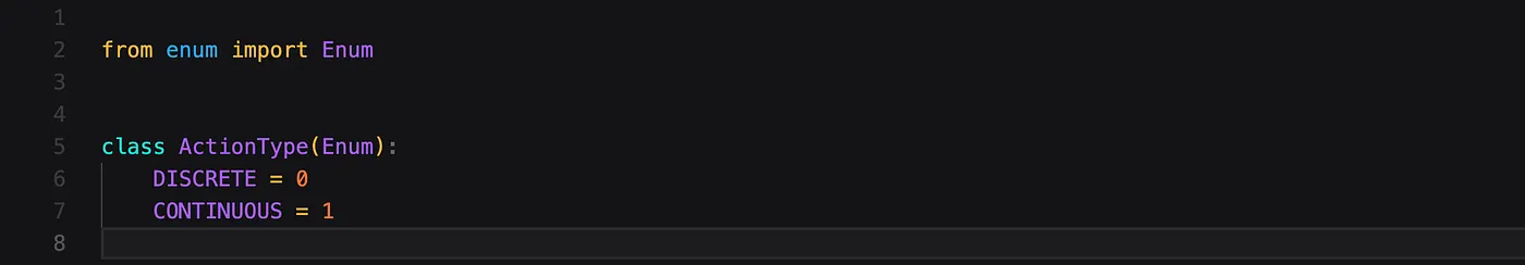
We define an ActionType enum, to make a distinction between environments that require a discrete action space or a continuous action space.
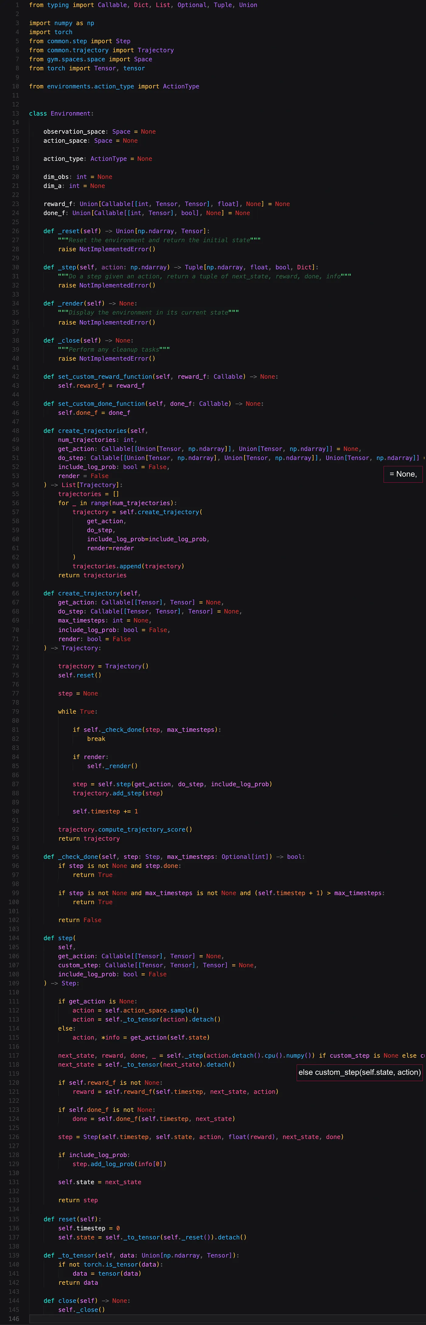
The next class is our actual environment abstraction. We define some variables like the dimensions of the state space (note: currently only vectors are supported), the dimensions of the action space and the type of actions, along with the usual Gym abstractions. We also allow the user to pass some functions as parameters. They allow a user to override the reward-function or how to determine when an episode is over.
The two most important functions are create_trajectory and step. The former will output a trajectory in the environment, the latter takes a single step in the environment. Both might be useful under certain circumstances.
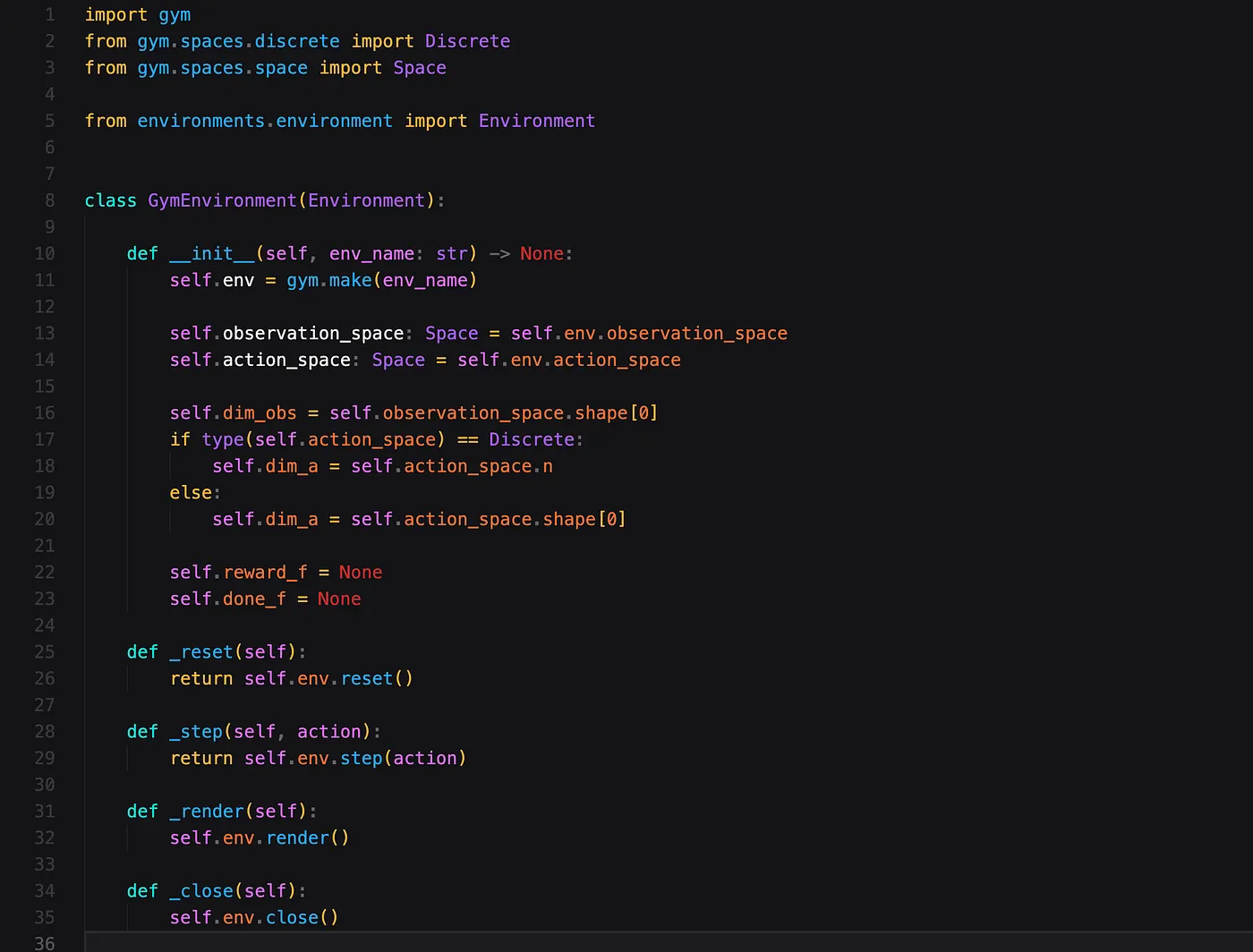
If you want to use this class in tandem with one of the environments provided by OpenAI Gym, you can do so with the following class, which inherits from the Environment class.
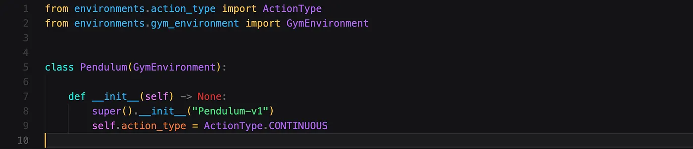
In order to use this with one of the environments, for example the Pendulum-environment, you can do it similar to this example.
Baseline calculation
As we have seen in the previous blogpost, we will also need to calculate the reward-to-go. I’ve made this code part of a file called “advantages.py”, since this value should in theory be similar to the advantage and we might want to reuse it later for other algorithms.
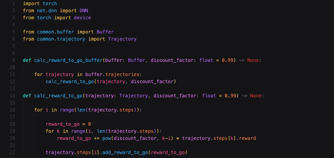
The file also mentions a buffer, which we will later use for other algorithms, but you can safely ignore it for now. The reward-to-go calculation takes a trajectory and a discount_factor as input. You might want to tweak the discount factor depending on how (un)important future rewards are for the problem you are solving.
Logging
To make sure that we see some output and can track how our RL agent is doing, we will write a class that performs some evaluation.
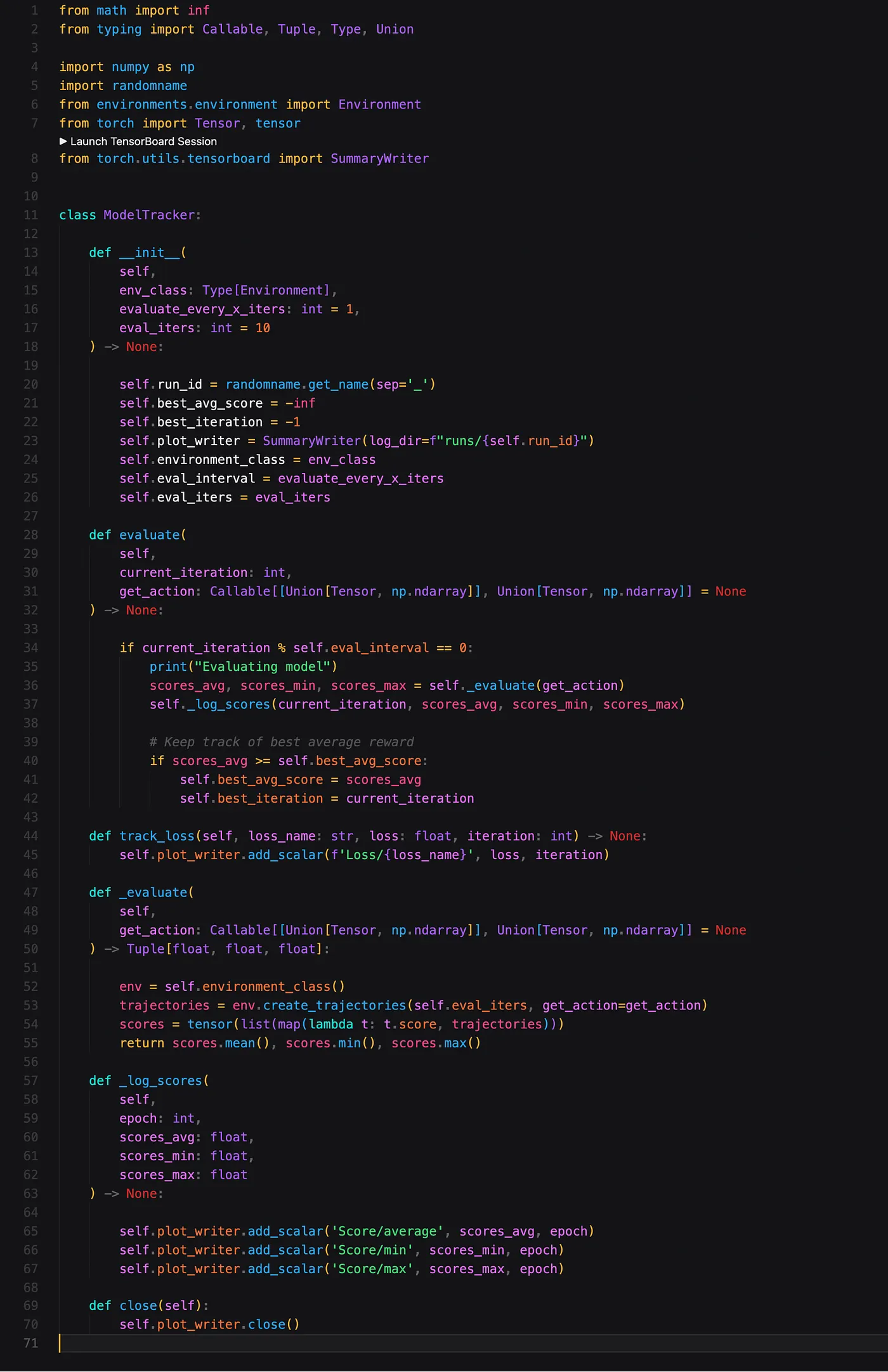
As you can see, we use the Tensorboard library in this class. This will allow us to track the progress of our algorithm through a nice dashboard with some graphs.
The crux of the logger is in the _evaluate function. Here we make use of the Environment class to create several trajectories. In order to create those trajectories, we pass in a parameter called get_action. The get_action parameter is a function that takes a state as input, and produces an action as output. This may seem very generic, and it is, but this is exactly the way we want it to allow maximum flexibility in what we want to evaluate.
Typically the get_action parameter will be a function that uses our RL agent to determine what the next action (given the state) should be.
Reinforce algorithm
We then arrive at the implementation of the actual algorithm. In this version we only sample one trajectory before every gradient update. It is definitely not wrong to sample multiple trajectories before doing a gradient update.

The most important part of this file is in the train function. First we initialise our environment and logger. We then sample a trajectory, for which we calculate the log probabilities of the taken actions, as well as the reward-to-go.
As you can see, we use some to_tensor functions, which are converting our array outputs to PyTorch Tensors for speedy calculations. In addition we call the to_device function which allows us to do some of the calculations on our graphics card instead of the CPU. For our purposes, these are just implementation details.
Next, we calculate the loss (target) by multiplying the log probabilities of the actions by the reward-to-go, as we have seen in the previous blog post. By default, PyTorch accumulates gradients, so we first call the zero_grad function to reset them. We then calculate the gradient of our loss with the backward function and update the weights with the step function.
In addition, this class contains some functions to save and load a trained model, and to sample an action from the model or sample an action deterministically.
Putting it all together
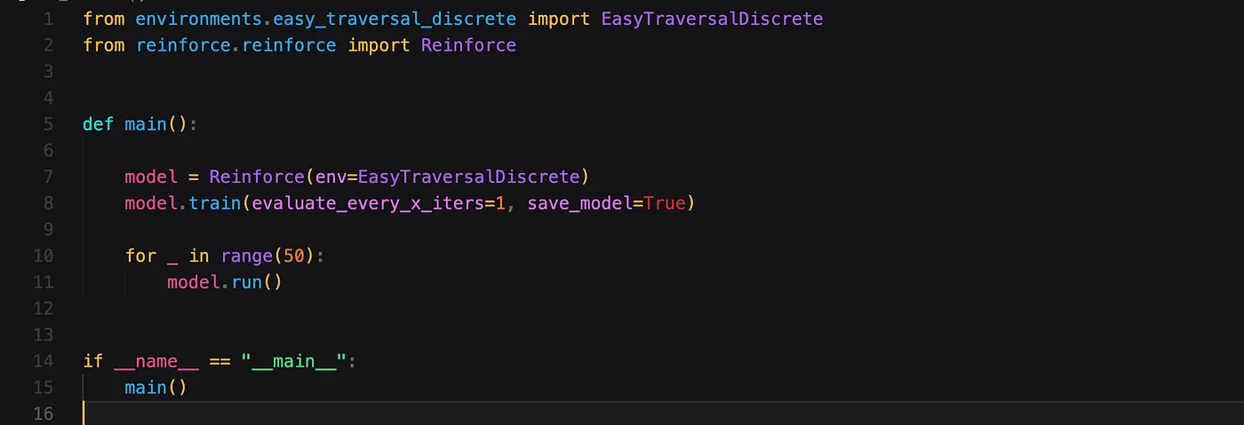
We now have all the ingredients to run our algorithm. I created a small main function that instantiates our Reinforce algorithm and passes in a custom environment called EasyTraversalDiscrete. We train the model using the default number of iterations and finally run our model!
For completeness, I will show what the directory structure of our project will look like. As you can see the project contains some extra files that we haven’t discussed yet, for now you can see these as a teaser for the following tutorials.

Conclusion
If you made it all the way here, congratulations, you have implemented your first RL algorithm and are probably well equipped to do your own research to explore more methods and algorithms.
The last part of this tutorial was probably not so easy to follow though, I have exclusively included images such that you would also think about what we are doing in the code, instead of blindly copying the code. If you have any questions though, feel free to leave a comment or to reach out to me personally.
Lastly, the files in this project are ordered in such a way, such that they allow for extending the code to other algorithms as well. This will be it for now however, so thank you for following this first series and see you in the next one!