Building a lane detection system using Python 3 and OpenCV
I started the Udacity Self Driving Car Engineer Nanodegree in December and it has been an absolute blast so far. Currently, I’m wrapping up my second project for classifying traffic signs using a convolutional neural network that employs a modified LeNet architecture. If you’re interested, you can check out my post about it here. I wanted to go back to my first project, detecting lane lines using OpenCV, and show anyone who might be interested in rudimentary computer vision exactly how it works and what it looks like. This was such a great project to start with as someone who was new to computer vision. I learned a lot and ultimately built a pipeline that works. You can find the code on GitHub. I highly encourage you to try the code out for yourself — you can even run it on your video!
The Challenge:
When we drive, we use our eyes to decide where to go. The lines on the road that show us where the lanes are act as our constant reference for where to steer the vehicle. Naturally, one of the first things we would like to do in developing a self-driving car is to automatically detect lane lines using an algorithm.
We want to start with an image like this:

Process the image for lane detection:

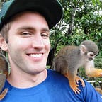
And finally extrapolate and average those lines for a smooth lane detection feature which we can apply to video frames:

The Approach:
The first step to working with our images will be to convert them to grayscale. This is a critical step to using the Canny Edge Detector inside of OpenCV. I’ll talk more about what canny() does in a minute, but right now it’s important to realize that we are collapsing 3 channels of pixel value (Red, Green, and Blue) into a single channel with a pixel value range of [0,255]. gray_image = cv2.cvtColor(image, cv2.COLOR_BGR2GRAY)

Before we can detect our edges, we need to make it clear exactly what we’re looking for. Lane lines are always yellow and white. Yellow can be a tricky color to isolate in RGB space, so lets convert instead to Hue Value Saturation or HSV color space. You can find a target range for yellow values by a Google search. The ones I used are below. Next, we will apply a mask to the original RGB image to return the pixels we’re interested in.
lower_yellow = np.array([20, 100, 100], dtype = “uint8”)
upper_yellow = np.array([30, 255, 255], dtype=”uint8")mask_yellow = cv2.inRange(img_hsv, lower_yellow, upper_yellow)
mask_white = cv2.inRange(gray_image, 200, 255)
mask_yw = cv2.bitwise_or(mask_white, mask_yellow)
mask_yw_image = cv2.bitwise_and(gray_image, mask_yw)

We are almost to the good stuff! We’ve certainly processed quite a bit since our original image, but the magic has yet to happen. Let’s apply a quick Gaussian blur. This filter will help to suppress noise in our Canny Edge Detection by averaging out the pixel values in a neighborhood.
kernel_size = 5
gauss_gray = gaussian_blur(mask_yw_image,kernel_size)
Canny Edge Detection
We’re ready! Let’s compute our Canny Edge Detection. A quick refresher on your calculus will really help to understand exactly what’s going on here! Basically, canny() parses the pixel values according to their directional derivative (i.e. gradient). What’s left over are the edges — or where there is a steep derivative in at least one direction. We will need to supply thresholds for canny() as it computes the gradient. John Canny himself recommended a low to high threshold ratio of 1:2 or 1:3.
low_threshold = 50
high_threshold = 150
canny_edges = canny(gauss_gray,low_threshold,high_threshold)
We’ve come a long way, but we’re not there yet. We don’t want our car to be paying attention to anything on the horizon, or even in the other lane. Our lane detection pipeline should focus on what’s in front of the car. Do do that, we are going to create another mask called our region of interest (ROI). Everything outside of the ROI will be set to black/zero, so we are only working with the relevant edges. I’ll spare you the details for how I made this polygon — take a look in the GitHub repo to see my implementation. roi_image = region_of_interest(canny_edges, vertices)

Hough Space
Prepare to have your mind blown. Your favorite equation y=mx+b is about to reveal its alter ego —the Hough transform. Udacity provides some amazing video content about Hough space, but it’s currently for students only. However, this is an excellent paper that will get you accquainted with the subject. If academic research publications aren’t your thing, don’t fret. The big take away is that in XY space lines are lines and points are points, but in Hough space lines correspond to points in XY space and points correspond to lines in XY space. This is what our pipeline will look like:
- Pixels are considered points in XY space
hough_lines()transforms these points into lines inside of Hough space- Wherever these lines intersect, there is a point of intersection in Hough space
- The point of intersection corresponds to a line in XY space
If you’re interested in the code for this portion, be sure to follow along in the Jupyter notebook in the repo. You can find more information the parameters for the Hough transform here. Don’t be afraid to experiment and try different thresholds! Let’s see what it looks like in action:

The key observation about the image above is that it contains zero pixel data from any of the photos we processed to create it. It is strictly black/zeros and the drawn lines. Also, what looks like simply two lines can actually be a multitude. In Hough space, there could have been many, many points of intersection that represnted lines in XY. We will want to combine all of these lines into two master averages. The solution I built to iterate over the lines is in the repo.
Once we have our two master lines, we can average our line image with the original, unaltered image of the road to have a nice, smooth overlay. complete = cv2.addWeighted(initial_img, alpha, line_image, beta, lambda)

Processing Video
It’s a few short lines to edit one frame, to creating a rolling average and processing 30FPS.
The Results:
This was a fantastic introduction to the Udacity SDC Engineer Nanodegree. I had a lot of fun working through this project and building my solution. That said, there are a few things I’d like to improve on.
- The lane detection region of interest (ROI), must be flexible. When driving up or down a steep incline, the horizon will change and no longer be a product of the proportions of the frame. This is also something to consider for tight turns and bumper to bumper traffic.
- Driving at night. The color identification and selection process works very well in day light. Introducing shadows will create some noisy, but it will not provide as rigorous a test as driving in night, or in limited visibility conditions (e.g. heavy fog)
In the meantime, I’ll be building a convolutional neural network to classify traffic signs, learning more about TensorFlow, and getting familiar with Keras. Stay tuned!