Fruit Image Classification
By: Hannah Li, Trisha Paul, Puja Subramaniam, and Shelby Watson
Abstract
In this blog, we will show our approach to classifying images of fruit using various supervised models. We identify a business problem and its relevance, and use a dataset obtained from Kaggle in order to perform our analyses. We discuss various data preprocesses we went through in order to reduce the dimensionality of the data, and to feed our models the best inputs possible. Next, we run models ranging in terms of complexity to find the best classifier of our fruit. Finally, we discuss the applications of our work and some ways it can be continued further.
Introduction
Grocery stores constantly strive to make sure their inventory and sales numbers are accurate. With such small margins being made on each item (typically just a few cents per item), it is important to make sure the price charged is precise in order to minimize loss. This can get tricky when it comes to produce. Parsley and cilantro look incredibly similar, and the differences between a honeycrisp and gala apple are not super obvious. When the wrong numbers are punched in for produce, a store can lose money and a customer could potentially pay too much or too little. This can lead to massive loss for stores, whether it be a loss of money or customer satisfaction.
We asked the question, “What if grocery store retailers didn’t have to have cashiers and customers manually identify produce?” This could reduce the loss associated with incorrectly identifying fruit, and could reduce waste by eliminating the need for stickers and labels on produce. To set out on our journey with fruit classification, we obtained an image dataset of fruits from Kaggle that contains over 82,000 images of 120 types of fruit.
Our dataset is contained in the fruits.zip file which can be downloaded here.
When starting our project, we knew from the get-go that a convolutional neural network would most likely be the best model for image classification. However, we decided to run several types of supervised learning models to see what we might find. Our selected models in addition to CNN include K Nearest Neighbors, Decision Trees, Random Forests, and VGG16, all of which we will discuss in further detail in our analysis. Before we began any of that, however, we needed to preprocess our data (a task not fit for the weary).
Loading Images
Unzip fruits and store image in train/test set:
with ZipFile('fruits.zip', 'r') as zipObj:
    listOfiles = zipObj.namelist()fruits_train = []
for mystring in df['image path']:
    if 'Training' in mystring:
            fruits_train.append(mystring)
fruits_train = pd.DataFrame(fruits_train, columns = ['image path'])#add label to image in dataframe
res = []
for i in fruits_train['image path']:
    res.append(re.findall("Training/(nt|[a-zA-Z\s+]+)", i)[0])
fruits_train['label'] = res
Store training set x features as images, and target as list of labels:
fruit_images = []
labels = []for i in range(len(fruits_train)):
    #read in image in color
    image = cv2.imread(fruits_train['image path'][i], cv2.IMREAD_COLOR)
    image = cv2.resize(image, (45, 45))
    #inverse image colors to show appropriately on screen (RGB to BGR)
    image = cv2.cvtColor(image, cv2.COLOR_RGB2BGR)
    fruit_images.append(image)
    labels.append(fruits_train['label'][i])#array of fruit images
fruit_images = np.array(fruit_images)#creating labels for images
labels = np.array(labels)
label2id = {v:i for i,v in enumerate(np.unique(labels))}
label_ids = np.array([label2id[x] for x in labels])
Data Preprocessing
Data preprocessing is a very, if not the most, important step in machine learning. Excess noise or missing values can skew the results of our dataset, so it is critical to preprocess our data so we can avoid these mishaps and improve our training time and accuracy.
Feature Extraction
Our dataset consists of 60,498 training images and 20,622 test images. Each image is 100x100, and each pixel has R, G, and B variables — this means each image has 30,000 features! This dataset is extremely high dimensional, so it is crucial to reduce the number of dimensions we are working with. This is important because not only will it save time and money (not to mention make the dataset much easier to run), but will also avoid overfitting the data. One way to do this is by performing feature extraction. Feature extraction creates a smaller set of new features that can accurately represent the current features in a dataset.
PCA
For our dataset, we used Principal Components Analysis (PCA). PCA is a linear dimension reduction technique that uses orthogonal projections to represent correlated variables into fewer uncorrelated variables, known as principal components. This technique allows our dataset to be represented the same while preventing the curse of dimensionality, and greatly reducing the number of dimensions/features in our dataset. This was especially helpful in understanding our data since we have so many features per image and a large amount of images.
Scree Plot
In order to know whether PCA will be useful or not, we need to create a scree plot. A scree plot shows the number of components plotted against explained variance. We want to use PCA if a low number of components has a high cumulative explained variance. The plot below shows that using PCA is beneficial, and as a result, we are able to reduce our dataset to 50 components with 99.79% variance retained.
scaler = StandardScaler()images_scaled = scaler.fit_transform([i.flatten() for i in fruit_images])pca = PCA().fit(images_scaled)


To visualize what PCA does, here is a sample of 400 images from the fruit dataset, untouched:

Here is the same sample with PCA (50 components) performed:

Here, we can see that the images are much more blurred and undefinable. This is because these images only have 50 components each, instead of 30,000. Although identifying the fruits in this plot is difficult for the human eye, our PCA model identifies these fruits nearly the same as if they were untouched — this is the beauty of PCA.
TSNE (t-distributed Stochastic Neighbor Embedding)
Since PCA is a linear dimension reduction technique, we were only able to visually plot the first two components. In order to remedy this, we used a TSNE plot. TSNE is a non-linear dimension reduction technique which allowed to represent all 50 PCA components we obtained, in 2 dimensions. TSNE can do dimension reduction just like PCA, but in this case, we used TSNE solely for visual purposes (to represent our results from PCA).
The code below demonstrates how we represented our PCA results in 2 dimensions:
tsne = TSNE(n_components=2, perplexity=40.0)
tsne_result = tsne.fit_transform(pca_result)
tsne_result_scaled = StandardScaler().fit_transform(tsne_result)tsnedf = DataFrame()
tsnedf['x'] = list(tsne_result_scaled[:,0])
tsnedf['y'] = list(tsne_result_scaled[:,1])
tsnedf['label'] = labels

Below is the code to run the TSNE plot:
nb_classes = len(np.unique(label_ids))
sns.set_style('white')
cmap = plt.cm.get_cmap("Spectral", 120)plt.figure(figsize=(20,20))
for i, label_id in enumerate(np.unique(label_ids)):

    #plot matching labels to tsne results so labels are accurate
    plt.scatter(tsne_result_scaled[np.where(label_ids == label_id), 0],
                tsne_result_scaled[np.where(label_ids == label_id), 1],
                marker = '.',
                c = cmap(i),
                linewidth = '5',
                alpha=0.8,
                label = id2label[label_id])
plt.title('T-SNE Plot (PCA 50 Components)', fontsize = 15)
plt.xlabel('X', fontsize = 15)
plt.ylabel('Y', fontsize = 15)
plt.legend(loc = 'center left', bbox_to_anchor = (1, 0.5), ncol = 2)
plt.show()

To better visualize our results, we created the same TSNE plot as above but using the actual images of the fruit. Here is the code to run the TSNE image plot:
#tsnedf is the dataframe as pictured above
#fruit_images is the array of imagesfig, ax = plt.subplots(figsize=(20,20))
for df, i in zip(tsnedf.iterrows(), fruit_images):
    x = df[1]['x']
    y = df[1]['y']    img = OffsetImage(i, zoom = .4)
    ab = AnnotationBbox(img, (x,y), xycoords = 'data', frameon = False)
    ax.add_artist(ab)
ax.update_datalim(tsnedf[['x', 'y']].values)
ax.autoscale()
plt.title('T-SNE Plot (PCA 50 Components)', fontsize = 15)
plt.xlabel('X', fontsize = 15)
plt.ylabel('Y', fontsize = 15)
plt.show()

From the plots above, we saw that the fruits remain clustered together, and we were able to represent our images in 50 dimensions without losing any variance. Next, we moved onto running our models using the results obtained from PCA.
Models
Train/Validation Split
In order to test and tune our models, we created train/validation sets using our PCA training dataset:
#getting pca results into dataframe
pcadf = DataFrame()
for i in range(50):
    pcadf[i] = pca_result[:,i]#creating train/validation (test) set
X_train, X_test, y_train, y_test = train_test_split(pcadf, label_ids, test_size=0.40, random_state=42)
Test Set
Use the code below to extract the test set images from fruits.zip and store into an array:
fruit_images_test = []
test_labels = []
for i in range(len(fruits_test)):
    image = cv2.imread(fruits_test['image path'][i], cv2.IMREAD_COLOR)
    image = cv2.resize(image, (45, 45))
    image = cv2.cvtColor(image, cv2.COLOR_RGB2BGR)
    fruit_images_test.append(image)
    test_labels.append(fruits_test['label'][i])
fruit_images_test = np.array(fruit_images_test)#creating labels for images
test_labels = np.array(test_labels)
test_label2id = {v:i for i,v in enumerate(np.unique(test_labels))}
test_label_ids = np.array([test_label2id[x] for x in test_labels])
KNN
After completing PCA, we wanted to see how well some “vanilla” models would perform on image classification. We started with K-Nearest-Neighbors, or KNN. KNN is used to classify and group images together. You might be thinking — how is this any different from what PCA did? The beauty of KNN is that it can actually predict where new fruits will be grouped. For example, if we introduce a new picture of a watermelon, a properly trained KNN model would be able to take this picture and group it along with other watermelons that we have in our dataset.
To start, we first created the model using sklearn’s KNeighborsClassifier. We didn’t know how many neighbors we would need in order to predict the label yet, so we wanted to test as many values as we could. We tested 1 to 200, in increments of 5. We then fitted the model to our training set, and predicted on our test set.
acc = []
for i in range(1, 200, 5):
    knn = KNeighborsClassifier(n_neighbors = i)
    knn.fit(X_train, y_train)
    y_pred = knn.predict(X_test)
    acc.append(accuracy_score(y_test, y_pred))

Our goal was to pick k to have the highest accuracy on our test set. We use accuracy here, instead of the preferred precision, because sklearn has a nice feature for multilabel classification where it is able to compute subset accuracy specifically. This gives us the positive predicted value — in simple terms, it tells us out of the labels the model predicted, how many of these were actually correct. As it turns out, this happened to be when k = 1. While it may appear that we are overfitting our data by only looking at 1 nearest neighbor, the reason we have the highest accuracy for this k value is because we had already completed a huge step in the process of clustering by performing PCA. Our data was already grouped by fruit label, so we did not have to look far to find the nearest neighbor that would accurately predict the fruit class.
From here, we were ready to predict on our test data. We went through the same preprocessing mentioned above to make sure that the features being used by the model were in the same format as the training data. After transforming the images, running PCA, and fitting the PCA components into the dataframe, we ran the model using KNeighborsClassifier from sklearn.
knn = KNeighborsClassifier(n_neighbors = 1)
knn.fit(X_train, y_train)
y_pred = knn.predict(X_test)
precision = (accuracy_score(test_label_ids, y_pred))*100
print("Accuracy with KNN: {0:.2f}%".format(precision))
We tested on the test data set, and calculated the accuracy of the model. In simple terms, it showed us how many of the labels our model predicted were correct. KNN actually performed well for us, with an accuracy of 94.49%. One of the downfalls of KNN is generally that it is sensitive to irrelevant features; this makes feature extraction super important. Given that we were able to successfully render our data through PCA, we could almost set it up perfectly for KNN. Ensuring a good combination of both data preprocessing as well as selecting an optimal K enabled us to create a high-performing KNN model.
Decision Trees
Next, we moved on to another very popular model — decision trees. Decision trees are pretty intuitive in that they split the data based on certain features that differentiate different groups. The splitting attributes determine the nodes of the tree, and the leaves tells us the label of fruit for each test set example.
We once again started by determining the optimal parameters for our tree. We fit the data to our training set using sklearn’s DecisionTreeClassifier, testing to see what the best depth of our tree would be (how many layers the tree has). We tested the range from 1–200 in intervals of 5, and get the best max_depth value of 36, as seen in the table and graph.
dtacc = []
for i in range(1,200, 5):
    dtree = DecisionTreeClassifier(max_depth = i)
    dtree.fit(X_train, y_train)
    y_pred = dtree.predict(X_test)
    dtacc.append(accuracy_score(y_test, y_pred))

dtree = DecisionTreeClassifier(max_depth = 36)
dtree.fit(X_train, y_train)
y_pred = dtree.predict(X_test)
precision = accuracy_score(y_pred, y_test)*100
print("Accuracy with Decision Tree: {0:.2f}%".format(precision))
With these parameters, we ran the model on our test set, and achieved a prediction accuracy of 74.92%. This accuracy may seem low, especially in comparison to what we were able to achieve with KNN. However, it’s good to keep in mind that our dataset is extremely large, and since we’ve done PCA as well, this is a pretty good accuracy score for a decision tree. While we are able to properly classify almost ¾ of the fruits, decision trees do have a disadvantage in that they take a long time to run, especially since our dataset is so large. Because of this, we decided to move on to random forests.
Random Forest
Random Forests build a larger number of individual trees, which helps to improve the accuracy of the prediction. One of the benefits of random forest is that it can handle large input variables with high dimensionality — this makes it a great classifier for our fruits! The model is able to do this using bootstrapping, where it samples from the images within our training set to determine the optimal max depth of each tree, given a set number of 100 trees within the forest. Fitting the model to our training set using sklearn’s RandomForestClassifier, gave us the following:


rf = RandomForestClassifier(max_depth = 46)
rf.fit(X_train, y_train)
y_pred = rf.predict(X_test)
precision = accuracy_score(y_pred, y_test)*100
print("Accuracy with Random Forest Tree: {0:.2f}%".format(precision))
We see that the validation accuracy starts to stabilize at about 99.8%, when we have a max depth of 46. This would change if we were to change the total number of trees in our forest.
The next step was to run the random forest model on our test data to see how well it could classify these fruits. We were able to achieve a test accuracy of 85.09%, which is higher than what we got using our decision tree model. While the decision tree we built had a few errors causing the accuracy to be lower, random forest is able to build multiple trees that consequently are able to cancel out errors in the others, thus reducing variance and stabilizing the model.
CNN
The next model we explored was a convolutional neural network (CNN). CNNs have hidden layers called convolutional layers, where filters are applied to detect the various patterns that exist in each image passed through the model. As the image goes deeper into the network, the pattern detection gets significantly more sophisticated. For example, those filters can detect specific objects such as eyes or scales on pictures of animals.
Within each convolutional layer, the number and size of filters and the stride size need to be specified. In our case, we are applying our filter and stride to get it to an appropriate convolved feature size for the next layer. After each convolutional layer, an additional activation function needs to be introduced to signal which node to go to in the next layer. ReLU is most commonly used, but others include tanh and sigmoid. After that, there is a pooling layer that applies an operation (most commonly the max operation) to each feature map. This outputs a matrix that reduces the dimensions without losing important feature information.
After pooling, the result gets sent to the next layer and the process is repeated through each of the layers. The results from the last pooling layer becomes the input for the fully connected layer. This layer is a traditional multilayer perceptron that uses a softmax activation function. The purpose of this layer is to use the features detected from the previous layers to classify the input image into its appropriate class based on the network and training set.
Our CNN Model
Given CNN’s ability to classify images well, we decided to apply this model to our dataset. Our CNN had four convolutional layers with the first layer having 16 filters, second layer having 32 filters, third layer having 64 layers, and fourth layer having 128 filters. For each layer, we added the ReLU activation function and used the max operation for pooling to reduce the spatial dimensions. For the fully connected layers, we used the softmax activation function, which is specifically used for multilabel classification. We ran our model with 20 epochs, with batch sizes of 120.
# specifying parameters for each convolutional layer
model = Sequential()
model.add(Conv2D(filters = 16, kernel_size = 2,input_shape=(100,100,3),padding='same'))
model.add(Activation('relu'))
model.add(MaxPooling2D(pool_size=2))
model.add(Conv2D(filters = 32,kernel_size = 2,activation= 'relu',padding='same'))
model.add(MaxPooling2D(pool_size=2))
model.add(Conv2D(filters = 64,kernel_size = 2,activation= 'relu',padding='same'))
model.add(MaxPooling2D(pool_size=2))
model.add(Conv2D(filters = 128,kernel_size = 2,activation= 'relu',padding='same'))
model.add(MaxPooling2D(pool_size=2))# specifying parameters for fully connected layer
model.add(Dropout(0.3))
model.add(Flatten())
model.add(Dense(150))
model.add(Activation('relu'))
model.add(Dropout(0.4))#last layer -- 120 for 120 classes
model.add(Dense(120,activation = 'softmax'))
model.summary()
Here is the result of our CNN model:
Our CNN model finished running after approximately one hour, resulting in a validation accuracy of 100% and a test accuracy of 98.92%.

Since our CNN weights are trained on our dataset, we are able to achieve a high accuracy even with a low number of epochs. After the second epoch, there is a significant increase in accuracy, which remained pretty constant throughout the remaining epochs.
VGG16
To add to our neural network models, we decided to apply transfer learning with a VGG16 model, which is similar to a CNN model. Transfer learning is a machine learning method in which a model that has already been developed is reused as the starting point model for another task. Since transfer learning models require a lot of time and computing power to train, we wanted to see if the results could justify the resources needed to run it. Some drawbacks to VGG16 are that it is slow to train, and the network architecture weights are large. Even though it is slow, the model is known to generally produce great results.
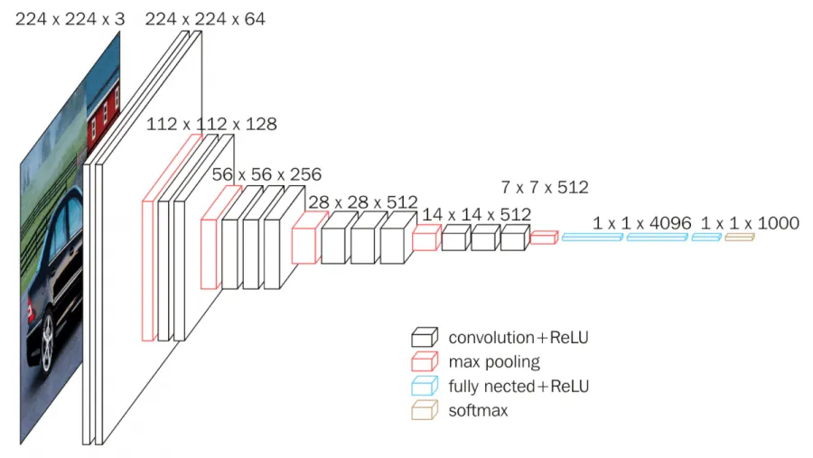
Our VGG16 Model
vgg = VGG16(input_shape=[100,100,3], weights='imagenet', include_top=False)
for layer in vgg.layers:
   layer.trainable = False
x = Flatten()(vgg.output)
prediction = Dense=(120, activation='softmax')(x)
We specified the input shapes for our VGG16 model to be 100x100x3. The pre-trained weights were extracted using ImageNet, and the softmax activation function was used for the last layer. We experimented with various steps per epoch, and found that 100 steps gave us a decent accuracy in a reasonable amount of time.


After six hours of running, the VGG16 model obtained a validation accuracy of 93.2%.This accuracy is actually lower than that of CNN, which may seem surprising at first. However, VGG16 trains on ImageNet, which is a database of general images; this makes it more noisy than our CNN model, which only trained on our fruit data.
Conclusion
Through our analyses, we were able to develop several models that classify fruits based on an image. Given the nature of our dataset, it was crucial that we first started by preprocessing our data. By implementing PCA, which reduced the dimensionality of our dataset, we were able to achieve high accuracies, even with our “vanilla” models. From there, we developed more complex neural networks, which gave us our best accuracy scores.

Not only do our models classify our own fruit dataset well, but they can also be generalized to other datasets, making our analysis applicable to a variety of settings. Utilizing neural networks made it easier to further train and increase accuracy, and over time, images with more noise could be added to train our models to classify the fruit in the noisy image. Also, more fruits and vegetables can be added and trained- even things like seeds, nuts, breads and pastries could be added for classification purposes. While our highest performing model is currently a CNN, the VGG16 model might be the best for long-term classification as more images are trained in the larger ImageNet database. Additionally, it is valuable to note that although KNN has a slightly lower accuracy than CNN, it took much less time to run. On the other hand, VGG16 took the longest to run and was only the third highest accuracy. Although the time-to-accuracy trade-off may not seem worth it in our case, VGG16 will likely become a better model as we expand our dataset to different, noisier images.
Over the course of our interactions in with this data, we learned the importance of dimensionality reduction and experienced the curse of dimensionality firsthand. Our preprocessing and application of PCA ended up being crucial to our understanding of the data, and further emphasized the importance of preprocessing and the time necessary to do so. While selecting our models, we learned quite a bit about the inner workings of convolutional neural networks and their ability to perform well in image classification. In addition, we researched and learned about transfer learning, how it works, and how it can be used to expand and improve our work.
This project gave us an opportunity to get down and dirty with a variety of different models, many of which we learned about in various courses. As we learned more about neural networks, we realized how much computing power is truly required to run these models on a large dataset. A great next step would be to try to reduce run times for our CNN and VGG16 models, ideally on a cloud computing platform that could handle large amounts of data well and widen the capacity of the model’s ability to predict.
Link to our GitHub can be found here.
References
Using CNN from scratch to classify images
Title image provided by slidesgo