Batch Normalization — Speed up Neural Network Training
Neural Network — a complex device, which is becoming one of the basic building blocks of AI. One of the important issues with using neural network is that the training of the network takes a long time for effectively deep networks — even on GPUs, let alone CPUs.
Neural networks learn the problem using BackPropagation algorithm. By backpropagation, the neurons learn how much error they did and correct themselves, i.e, correct their “weights” and “biases”. By this they learn the problem to produce correct outputs given the inputs. BackPropagation involves computing gradients for each layer and propagating it backward, hence the name.

But during backpropagation of errors to the weights and biases, we’ll face a undesired property of Internal Covariate Shift. This makes the network too long to train.
Internal Covariate Shift
During training, each layer is trying to correct itself for the error made up during the forward propagation. But every single layer acts separately, trying to correct itself for the error made up.

For example, in the network given above, the 2nd layer adjusts its weights and biases to correct for the output. But due to this readjustment, the output of 2nd layer, i.e, the input of 3rd layer is changed for same initial input. So the third layer has to learn from scratch to produce the correct outputs for the same data.

This presents the problem of a layer starting to learn after it’s previous layer, i.e, 3rd layer learns after 2nd finished, 4th starts learning after 3rd, etc. Similarly, think of the current existing deep neural networks that are about 100 to even 1000 layers deep! It would really take epochs to train them :D
More specifically, due to changes in weights of previous layers, the distribution of input values for current layer changes, forcing it to learn from new “input distribution”.
Normalization
In a dataset, all the features (columns) may not be in same range. For eg. Price of house (thousands), Age of house (within 100) etc. It takes lot of time to train for these kind of datasets.

Usually, in simpler ML algorithms like linear regression, the input is “normalized” before training to make them into single distribution. Normalization is to convert the distribution of all inputs to have mean=0 and standard deviation=1. So most of the values lie between -1 and 1.
We can even apply this normalization to the input of neural networks. It fastens up training as in linear regression. But since the 2nd layer changes this distribution, the consecutive layers are not benefited. So, what can we do? Yeah! Why not add normalization between each layers? This is what Batch normalization does.
Batch Normalization
To reduce this problem of internal covariate shift, Batch Normalization adds Normalization “layer” between each layers. An important thing to note here is that normalization has to be done separately for each dimension (input neuron), over the ‘mini-batches’, and not altogether with all dimensions. Hence the name ‘batch’ normalization.
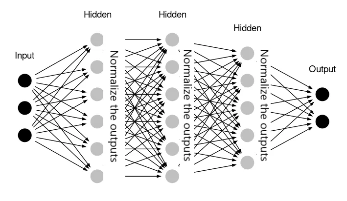
Due to this normalization “layers” between each fully connected layers, the range of input distribution of each layer stays the same, no matter the changes in the previous layer. Given x inputs from k-th neuron.

Normalization brings all the inputs centered around 0. This way, there is not much change in each layer input. So, layers in the network can learn from the back-propagation simultaneously, without waiting for the previous layer to learn. This fastens up the training of networks.
We apply Batch Normalization to the best-performing ImageNet classification network, and show that we can match its performance using only 7% of the training steps, and can further exceed its accuracy by a substantial margin. — Original BatchNorm Paper
Batch Normalization is great. But, there are a few minor issues with BatchNorm which we need to take care of.
Scale and Shift
There are usually two types in which Batch Normalization can be applied:
- Before activation function (non-linearity)
- After non-linearity
In the original paper, BatchNorm is applied before the applying activation. Most of the activation functions have problems while applied this way. For sigmoid and tanh activation, normalized region is more of linear than nonlinear.

For relu activation, half of the inputs are zeroed out.

So, some transformation has to be done to move the distribution away from 0. A scaling factor γ and shifting factor β are used to do this.

As training progresses, these γ and β also learn through backpropagation so as to improve accuracy. This imposes that 2 extra parameters be learnt for each layer to increase training speed.
This final transformation thus completes definition of Batch Normalization algorithm. Use of scaling and shifting is particularly much useful because, it provides more flexibility. Suppose if we decide not to use BatchNorm, we can set γ = σ and β = mean, thus giving back the original values.
Recently, it has been observed that the BatchNorm when applied after activation, performs better and even gives better accuracy. For such case, we may decide to use only BatchNorm alone and not scaling and shifting. For such, set γ = 1 and β = 0. Nevertheless, γ and β are included in Batch Normalization Algorithm.
BatchNorm at Inference time
We now know that Batch Normalization calculates mean and variance for each mini-batch at training time and learns using back-propagation. But, what to do at Inference time? It would not be ok if we are to use mean and variance of testing mini-batch, because it may be skewed.
What we do is, we calculate “population average” of mean and variances after training, using all the mini-batch mean and variances. And at inference time, we fix the mean and variance to be this value and use it in normalization. This provides more accurate value of mean and variance.

But, sometimes, it is difficult to keep track of all the mini-batch mean and variances. In such cases, exponential weighted “moving average” can be used to update population mean and variance:

Here α is the “momentum” given to previous moving statistic, around 0.9. And those with B subscript are mini-batch mean and mini-batch variance. This is the implementation found in most libraries, where the momentum can be set manually.
An important thing to note here is that the moving mean and moving variance are calculated at training time, with training dataset and not at testing time.
Regularization by BatchNorm
In addition to fastening up the learning of neural networks, BatchNorm also provides a weak form of regularization. How does it introduce Regularization? Regularization may be caused by introduction of noise to the data. Since the normalization is not performed on the whole dataset and just on the mini-batch, they act as noise.
However BatchNorm provides only a weak regularization, it must not be fully relied upon to avoid over-fitting. Yet, other regularization could be reduced accordingly. For example, if dropout of 0.6 (drop rate) is to be given, with BatchNorm, you can reduce the drop rate to 0.4. BatchNorm provides regularization only when the batch size is small.
This ends introduction to Batch Normalization. In the next post, I have explained how Batch Normalization layers can be used with Tensorflow and provided links to train neural network with and without Batch Normalization.
Please do comment about what you feel about this post.