Sentiment Analysis in Keras using Attention Mechanism on Yelp Reviews Dataset
Authors
Kushagra Gupta, Jeewon Kim, Arpitnagpal
Table of content
- Introduction and Motivation
- Sentiment Modeling problem
- Bi-LSTM with Attention Mechanism Explained
- Implementation with real-world data
Content
1. Introduction and Motivation
Sentiment analysis is a powerful marketing tool that enables product managers to understand customer emotions in their marketing campaigns. It is an essential factor in product and brand recognition, customer loyalty, customer satisfaction, advertising and promotional success, and product acceptance. Understanding the psychology of consumers can help product managers and customer success managers to alter their product roadmap with greater precision. The term emotion-based marketing is a broad umbrella phrase that encompasses emotional customer responses, such as “positive,” “negative,” “neutral,” “negative,” “uptight,” “disgust,” “frustration,” and others. Understanding the psychology of customer responses can also increase product and brand recall.
Analyzing product sentiment requires a solid understanding of how customers think. Keywords and phrases commonly used in customer service conversations can reveal product and brand insight. A product manager or a customer success can quickly identify negative and positive words used in product reviews using customer feedback analytics tools, which would indicate issues in product support. Likewise, specific keywords associated with product boosting can reveal marketing campaigns, such as “how to get more sales” or “make more money.” These insights help product managers determine which messages to deliver to customers.
To further understand the sentiment analysis technic, in this tutorial, we will classify the sentiment of Yelp reviews with a deep learning neural network model.
2. Sentiment Modeling problem
Sentiment Analysis is basically a recognition of an utterance’s emotional tone — in our case, the algorithm tells us whether a given statement is negative or positive:
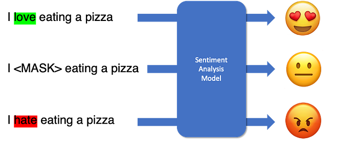
To conduct the stated classification task, there are several accessible solutions for analyzing the sentiment of the text, such as the VADER package and the Deep Neural Network model to classify the feeling of a given phrase.
3. Bi-LSTM with Attention Mechanism Explained
3–1) What is LSTM?
Humans do not start learning everything from the beginning; they basically relate things to each other to make inferences about the new thing in their minds. For example, when they learn how to ride a motorcycle, and they already know how to cycle, they don’t need to learn about braking or any other basic things because they already know them. They just add the extra information with the regular or older information. Traditional neural networks can’t do this. It’s a shortcoming of neural networks, and RNN(recurrent neural network) fixes this issue. They are networks with various loops to persist the information, and LSTM(long short term memory) is a special kind of recurrent neural network, which are very useful when dealing with sequential data like time series data and NLP data.
3–2) What is Bi-LSTM?
Bidirectional long short term memory (Bi-LSTM) is a type of LSTM model which processes the data in both forward and backward directions. This feature of data flow in both directions makes the BI-LSTM different from other LSTMs.
For example, consider the sentence ‘I love the movie, it was a fantastic feeling watching it’ and to classes like and hate. From the inference of the sentence, we need to classify which class it is related to. For this, a unidirectional LSTM models layer will go through ‘I love ……….watching it’ like this or ‘it watching ……….love i’ like this and persist the information in the sequences and bidirectional LSTM. The model layers the process of the sentence in both directions and persists the information of both types (start to end) and (end to start) so that whenever the words like love or fantastic come again in any sentence model can classify them as love class.
3–3) What is the Attention Mechanism?
The attention mechanism was introduced to improve the performance of the encoder-decoder model for machine translation. The idea behind the attention mechanism was to permit the decoder to utilize the most relevant parts of the input sequence in a flexible manner, by a weighted combination of all of the encoded input vectors, with the most relevant vectors being attributed to the highest weights.
In a nutshell, attention in deep learning can be broadly interpreted as a vector of importance weights: in order to predict or infer one element, such as a pixel in an image or a word in a sentence, we estimate using the attention vector how strongly it is correlated with (or “attends to” as you may have read in many papers) other elements and take the sum of their values weighted by the attention vector as the approximation of the target.
4. Implementation with real-world data
In the following tutorial, we will be using a bi-directional RNN with Attention instead of a vanilla unidirectional RNN. Despite the fancy name, this is simply the concatenation of two RNNs. One RNN processes the sequence from left to right (the “forward” RNN), while the other processes the sequence from right to left (the “backward” RNN). By using both directions, we get a more reliable encoding as each word can be given the context of its neighbours on both sides (rather than just earlier in the sequence).
4–1) Data Sourcing
We decided to utilize 200,000 Yelp Reviews from the dataset available on https://www.yelp.com/dataset. The Yelp dataset is a subset of Yelp businesses, reviews, and user data for use for personal, educational, and academic purposes. It’s available as JSON files, so institutions may use it to teach students about databases, learn NLP, or sample production data while you learn how to make mobile apps. Yelp open dataset contains various kinds of features and data as well, but we’ll be focusing on “the reviews” only for sentiment analysis.
4–2) Data Preprocessing
Once the data has been gathered, we had to read it and process it before passing it into the model.
To do so, we need to import required libraries such as NLTKs and dataset first.
import pandas as pd
import numpy as npimport nltk
nltk.download('stopwords')
nltk.download('wordnet')import re
from nltk.stem import WordNetLemmatizer
from nltk.corpus import stopwordsfrom sklearn.model_selection import train_test_split
import tensorflow as tf
import tensorflow.keras as keras
from tensorflow.keras.preprocessing.text import Tokenizer
from tensorflow.keras.preprocessing.sequence import pad_sequences
from tensorflow.keras.layers import Concatenate, Dense, Input, LSTM, Embedding, Dropout, Activation, GRU, Flatten
from tensorflow.keras.layers import Bidirectional, GlobalMaxPool1D
from tensorflow.keras.models import Model, Sequential
from tensorflow.keras.layers import Convolution1D
from tensorflow.keras import initializers, regularizers, constraints, optimizers, layersreview_json_path = r'C:\Users\Dell\Desktop\yelp_academic_dataset_review.json'
size = 200000
review = pd.read_json(review_json_path, lines=True,
dtype={'review_id':str,'user_id':str,
'business_id':str,'stars':int,
'date':str,'text':str,'useful':int,
'funny':int,'cool':int}, nrows=size)df_review_text=review[['stars','text']]
For problem modelling, we then need to define the sentiment as a target variable from the given dataset first. To do so, We look at the distribution of ‘the stars’ from the reviews.
df_review_text['stars'].value_counts(dropna=False).sort_index().plot(kind='bar')We can see that people are positive to mainly give 4 or 5 stars. Based on the observation, we decided to create a new feature sentiment with values 0 and 1. The reviews with stars above 3 are “positive”, with a value of 1. Others are “negative”, with a value of 0.
df_review_text['sentiment'] = np.where(df_review_text['stars'] > 3, 1, 0)It’s rarely the case that we get preprocessed numerical sequences representing text data. As such, we should pay attention to how our text is converted to the numbers that our attention model can understand.
For our raw text, we need to do some filtering before our model-building. In addition to filtering out punctuation characters, we also want to make everything lowercase. We also want to reduce words to just their root (e.g., so words like “jump” and “jumping” aren’t given widely different encodings) - So we are conducting ‘lemmatization’ on Yelp reviews as well.
stop_words = set(stopwords.words("english"))
lemmatizer = WordNetLemmatizer()def clean_text(text):
  text = re.sub(r'[^\w\s]','',text, re.UNICODE)
  text = text.lower()
  text = [lemmatizer.lemmatize(token) for token in text.split(" ")]
  text = [lemmatizer.lemmatize(token, "v") for token in text]
  text = [word for word in text if not word in stop_words]
  text = " ".join(text)
  return textdf_review_text['Processed_Reviews'] = df_review_text.text.apply(lambda x: clean_text(x))
As a result, we now have a preprocessed review alongside the target variable, ‘sentiment.’
Before we finally get into the modelling part, we need to split the dataset into test and train data, so that we can train the model and gauge its performance with each dataset.
from sklearn.model_selection import train_test_splitdf_train, df_test = train_test_split(df_review_text, test_size=0.01)MAX_FEATURES = 6000
EMBED_SIZE = 128
tokenizer = Tokenizer(num_words=MAX_FEATURES)
tokenizer.fit_on_texts(df_train['Processed_Reviews'])
list_tokenized_train = tokenizer.texts_to_sequences(df_train['Processed_Reviews'])RNN_CELL_SIZE = 32
MAX_LEN = 60   # Since our mean length is 56.6
X_train = pad_sequences(list_tokenized_train, maxlen=MAX_LEN)
y_train = df_train['sentiment']
4–3) Model development
Defining Attention
Our use of an attention layer solves a confusion with using RNNs. We can easily use the final encoded state of a recurrent neural network for a prediction task. However, given the tendency of RNNs to forget relevant information in the previous steps of the sequence, this could lose some of the useful information encoded there. In order to keep that information, we can use an average of the encoded states of the RNN outputs. Since all these encoded states of the RNN are equally valuable, we use a weighted sum of these encoded states to make our prediction.
class Attention(tf.keras.Model):
    def __init__(self, units):
        super(Attention, self).__init__()
        self.W1 = tf.keras.layers.Dense(units)
        self.W2 = tf.keras.layers.Dense(units)
        self.V = tf.keras.layers.Dense(1)

    def call(self, features, hidden):
        hidden_with_time_axis = tf.expand_dims(hidden, 1)
        score = tf.nn.tanh(
            self.W1(features) + self.W2(hidden_with_time_axis))

        attention_weights = tf.nn.softmax(self.V(score), axis=1)        context_vector = attention_weights * features
        context_vector = tf.reduce_sum(context_vector, axis=1)

        return context_vector, attention_weights
We’re computing these attention weights by building a small fully connected neural network on top of each encoded state. This network will have a single-unit final output layer that will correspond to the attention weight we will assign.
Our Attention function is multiple dense layers plus a tanh function.
Embedding Layer
To perform the computations on input sentences, we must first embed them as a vector of numbers. There are three main approaches to performing this embedding pre-trained embeddings like Word2Vec or Glove or randomly initializing.
To perform this embedding we use the Embedding function from the layers package. The parameters of this matrix will then be trained with the rest of the graph.
sequence_input = Input(shape=(MAX_LEN,), dtype="int32")
embedded_sequences = Embedding(MAX_FEATURES, EMBED_SIZE)(sequence_input)
Bi-Directional RNN
We will be using a bi-directional RNN instead of a vanilla unidirectional RNN. It is simply the concatenation of two RNNs. One RNN processes the sequence from left to right, while the other processes the sequence from right to left. By using both directions, we get a more reliable encoding as each word can be given the context of its neighbours on both sides.
lstm = Bidirectional(LSTM(RNN_CELL_SIZE, return_sequences = True), name="bi_lstm_0")(embedded_sequences)# Getting our LSTM outputs
(lstm, forward_h, forward_c, backward_h, backward_c) = Bidirectional(LSTM(RNN_CELL_SIZE, return_sequences=True, return_state=True), name="bi_lstm_1")(lstm)
Since our model uses a bi-directional RNN, we first concatenate the hidden states from each RNN before computing the attention weights and applying the weighted sum.
state_h = Concatenate()([forward_h, backward_h])
state_c = Concatenate()([forward_c, backward_c])context_vector, attention_weights = Attention(10)(lstm, state_h)
dense1 = Dense(20, activation="relu")(context_vector)
dropout = Dropout(0.05)(dense1)
output = Dense(1, activation="sigmoid")(dropout)model = keras.Model(inputs=sequence_input, outputs=output)
The last layer is densely connected with a single output node. Using the sigmoid activation function, this value is a float between 0 and 1, representing a probability, or confidence level. We can easily print a list of our layers in Keras. Below is a summary of our model.
In order to train our model, we need to give it a loss function and an optimizer. An out-of-the-box Adam optimizer will also be what we use to optimize our model. Since our model is a binary classification problem and the model outputs a probability we’ll use the standard binary_crossentropy loss function.
For the sake of model improvement, our optimizer will only focus on accuracy.
METRICS = [
      keras.metrics.TruePositives(name='tp'),
      keras.metrics.FalsePositives(name='fp'),
      keras.metrics.TrueNegatives(name='tn'),
      keras.metrics.FalseNegatives(name='fn'),
      keras.metrics.BinaryAccuracy(name='accuracy'),
      keras.metrics.Precision(name='precision'),
      keras.metrics.Recall(name='recall'),
      keras.metrics.AUC(name='auc'),
]model.compile(loss='binary_crossentropy', optimizer='adam', metrics=METRICS)
We’ll train our Attention model for 5 epochs in mini-batches of 100 samples. While training, monitor the model’s loss and accuracy on the 20% samples from the validation set.
BATCH_SIZE = 100
EPOCHS = 5
history = model.fit(X_train,y_train,
                    batch_size=BATCH_SIZE,
                    epochs=EPOCHS,
                    validation_split=0.2)
As you can see in the below image, our model managed to achieve a decent performance only after 5 epochs of training.
Evaluating the model
During the training epochs, True Negatives and True Positives rise, False Positives and False Negatives fall, Accuracy and AUC steadily rise, and the Precision and Recall tend towards 1.0. This was pretty good for the first try.
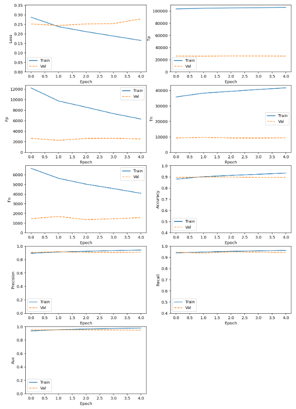
For evaluation purposes, we can further generate a list of predictions on previously unseen test data, and take a look into the ‘classification report’ and the ‘confusion matrix.’

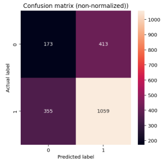
Overall our classifier is doing well, showing a 73% F1-score accuracy on the classifying positive review task from the test dataset.
You can find the full version of our code here.
Reference:
- https://www.linkedin.com/pulse/real-reasons-why-sentiment-analysis-important-2021-stefan-link/?trk=public_profile_article_view
- https://machinelearningmastery.com/the-attention-mechanism-from-scratch/
- https://lilianweng.github.io/posts/2018-06-24-attention/
- https://analyticsindiamag.com/hands-on-guide-to-bi-lstm-with-attention/
- https://voicelab.ai/explainable-artificial-intelligence-xai-in-sentiment-analysis/


