StyleGan Deep Dive: from its architecture to how to make synthetic humans

StyleGan (1,2,3) is considered State of the Art in image Synthesis for GANs, its architecture is fascinating and its applications are exiting.

14 min readOct 4, 2022

In this article we will learn:

What are GANs
How they work
The orginial objective loss function
In depth understanding of StyleGan
The mapping network
AdaIn
StyleMixing
Noise inputs
What dataset you can use
How to train it yourself, whith what parameters
And finally what results you can expect!

For a long time, Artificial Neural networks haven’t been able to produce satisfying enough results to be used as creation tools. Lately, with the emergence of powerful GANs and RNNs those technologies have become more and more famous. A few examples would be DALE and StyleGan.

GANs are Generative Adversarial Neural Networks but, what does this mean?

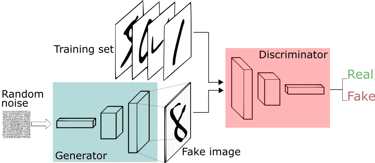
As the name suggests, in GANs there are two neural networks: a generator and a discriminator that are both competing in a zero-sum game to create artificial images.

The Generator starts with random noise (often from a Gaussian distribution) and is used to bootstrap the discriminator. The discriminator’s job is to discriminate real images from fake ones.

Very fast the discriminator gets good at saying if the image is fake or real, it only needs to discriminate random noisy pictures from, let’s say human faces.

But every time the discriminator makes a guess, we can compute the loss function and backpropagate it through the networks.

What is interesting is that even if those two neural networks are two fully differentiable we can still backpropagate this loss function across all pipeline.

To make things a bit clearer let’s quickly take a look at the original objective loss function from the original 2014 paper: Generative Adversarial Nets by Goodfellow, et al.

Ahhhh, looking at your face I almost spilled my tea 🍵 on my pants.

Don’t worry it looks scary but it is actually simple.

Let’s break it down

In this section, we can see that the Discriminator (D) has to maximize the value of X (output of discriminator), to make it as close as possible to 1,for all real images coming from our dataset.

Here G is the generator, and Z is the noise from our latent space which later in the training will become our fake images. Here we want to make all G(z) images recognized as fake, therefore outputting a low value close to zero.

So to sum up we want:

Real images to be output as 1 → D(X)
Fake images to be output as 0 -> G(Z)

This is the Min-Max game, you can see it at the beginning of the loss function.

We are trying to minimize the loss of the discriminator while maximizing the G(Z) output to make it as close as possible to 1 (real images).

In a perfect scenario, we consider that the Generator has won when the Discriminator is outputting 50% of the time that images are fake and 50% that they are real.

Now that you got a clearer understanding of how GANs are working and of the original objective loss function, let’s get to the fun part: StyleGan

The StyleGan paper, that you can find here is HUGE.

It is introducing a lot of different things, ranging from a dataset, new metrics, styleregulization, and new architecture. So let’s first sum up the key 🔑 new things StyleGan is bringing:

StyleGan architecture is bringing:

A new mapping framework called W
Affine Transformation (A) and Adaptive normalization (AdaIN) in the synthesis network
Multiple Noise inputs (B) throughout the layers of the synthesis network

The mapping network:

In normal GANs the random noise is first fed into what is called a latent space.

A latent space is a common way of processing data in machine learning, it is basically just compressed data represented using multidimensional vectors. It is often used in autoencoders. If you are not very familiar with it, that’s okay, I recommend this very good article from Ekin Tiu to better understand the concept.

But in styleGan instead of having this random latent vector (Z) being fed directly into the generator, there is the mapping network.

One of the issues of the Z vector is that it is randomly distributed, even where we don’t have data.

This is making the job of the generator way more complicated, it has to itself learn how to wrap the random data to avoid gaps.

It is pretty tricky to under, let’s take a look at this illustration from the paper:

a) represent the gap that we have in our data set, if we would have a human face dataset, we might have very few women with a beard. This is the empty square that you can see

b) represent how the feature would be mapped with a random Z distribution, the shape is very different from our real data shape and it has no gap

c) represent the learned mapped W vector, which looks more similar to our data and has the missing data gap

If we would use the b) example, with a random Z distribution the generator would have to learn the mapping function and wrap this Z distribution into a)

But with the mapping network, we create another simple network (chain of fully connected layers) whose job is to map the Z vector into a custom vector; W.

Now that we mapped the vector Z into W, we don’t directly feed this data at the beginning of the synthesis network, like on traditional GANs. (take a look at the figure again)

We will feed it later using the Affine Transformation (A) and the Adaptive normalization (AdaIN), the synthesis network actually starts with a constant distribution. A bit like a seed

AdaIN

The goal of feeding the W latent vector to the network by using the A and AdaIN is: disentanglement

StyleGan is called StyleGan for two reasons because it is highly inspired by style transfer literature. And because one of its goals is to separate styles (proprieties of the image).

You want the generator to be able to control the styles and modify them, for example modifying the eyes, the hair, or the face. Giving easily separable style to the generator allows StyleGan to generate very diverse images.

To do so we take the weights of our mapped vector W that we will call y, we feed them with x the convolutional features of the precedent layer from the synthesis network.

We then feed y and x into the Adaptive normalization (AdaIN) which is a mix of Batch Normalization and Instance Normalization.

If you’re not really comfortable with those two concepts it is okay, we will just be explaining the relevant part for Style control.

Again don’t be scared let’s take a look at what AdaIN actually does:

AdaIN is performing a normalization which is controlled by the weights of the W vector; ys,i and yb,i.

ys,i control the scale of the image, and yb,i control the translation. That’s why we say that AdaIN controls the styles of the image.

It basically takes the information from the convolutions of our synthesis network and combines it with our learned W latent vector.

By doing so at serval points on the synthesis network the generator can control and generate specific styles and disentangle them.

To be clearer the authors explain:

To be cleared the authors explain:

“We can view the mapping network and affine transformations as a way to draw samples for each style from a learned distribution, and the synthesis network as a way to generate a novel image based on a collection of styles”

Pheeeeeee…, I know this part is a bit abstract to represent, but you just need to remember this is were the styles of StyleGan are coming from.

So now we know how to disentangle the styles and we gave some control to the generator.

But to really able to control them, Stylegan is equipped with style regularization or StyleMixing.

StyleMixing

StyleMixing is a really interesting way of improving the FID (Fréchet inception distance), a common quality metric in GANs. But it is also a very fun image manipulation method.

The idea of StyleMixing is that if you take two vectors W1 and W2 you then feed them to the synthesis network at random layers at each training iteration.

The rule for the use of the W1 and W2 vectors is that the W1 vector is applied from the first layer to a specific layer called, the crossover point, where the W2 vector is then fed in till the end of the network.

This is allowing the network to learn that the adjacent vectors are not necessarily correlated.

The key thing 🔑 here is that if we change the crossover point, we can distinguish, low level styles from high levels ones, and control them!!

Look at this, it will make more sense:

Here we can observe different interesting things happening when we modify the crossover point (what layer we feed W1&W2):

Low res layers [4x4–8x8] (1st line): Here the low level attributes (eyes/hair/skin colors) are copied from A while the high levels attributes (pose, hairstyle, face shape) are copied from B
Medium res layers [16x16–32x32] (2sd line): High level attributes are copied from A and low level ones are copied from B
High res layers [64x64–1024x1024] (3rd line): All attributes are copied from A and only very small subtle details from B

We can see in this table that the Mixing regularization greatly improves the FID (Fréchet inception distance). The number of latent represents the number of W vectors that are used, and E and F are different configurations described in the paper.

You might wonder why there are different resolutions in the synthesis network. It all comes back to the earlier brother of StyleGan presented in a paper called Progressive Growing of GANs for Improved Quality, Stability, and Variation by Karras et all.

G here is the genrator and D the Discriminator. StyleGan kept the very efficient Generator of the Progressive Growing GAN.

Now let’s take a lot at the last particularity of StyleGan:

Noise inputs

Now let’s take a look at the noise inputs B, here instead of being fed at the beginning only, there are 4 noise vectors before each AdaIN normalization.

This noise vector allows StyleGan to integrate stochastic variation, which means that we input noise that follows a specific distribution. It is very useful for hairs, freckles, or skin details. It allows StyleGan to create diverse stochastic details in the pictures.

The main advantage of inputting those noise vectors before each AdaIN in the synthesis network is that in StyleGan the noise as said above only change subtle details. In regular GANs the noise inputs, totally change the image created.

This is a very smart way of integrating noise without compromising the style which is been created

Congrats! 🎉 — — We’re now done with the theory!

I hope that you now have a clear vision of how StyleGan is working and that you’re ready to run this incredibly clever 28 Million parameters neural network on your computer! (or online GPU)

First, let’s start with the dataset, yeah trust me it can take some time to download (even on Google Colab or Kaggle)

Datasets

I personally trained StyleGan2 (I will come back on this later) on 3 distinct datasets, here I will present 2 famous ones and 1 to experiment with:

First there is Flicker Face HQ Dataset

This is the dataset presented in the StyleGan paper, it’s a very high resolution [1024x1024] and diverse dataset (pose, skin color, age, clothes, etc) composed of 70,000 png images.

It is significantly better than the classic CelebA dataset, which wouldn’t take advantage of all the innovations we learned about above.

Secondly there is the Kaggle Abstract Art dataset

This is a pretty cool dataset, that you can find on Kaggle, it is probably extracted from the wikiart dataset.

It is composed of 28,820 images of abstract art in [512x512] resolution.

Art is a very cool use of GANs, abstract shouldn’t be too much challenging for stylegan.

Spoiler: During my tests, people that I asked couldn’t tell the difference between fake art and real one.

And in thrird there is the MetFace dataset

This dataset is also a face dataset. As we humans are very good at recognizing faces, asking a GAN to create faces creates a very intuitive benchmark for us.

It is made of 1336 high resolution [1024x1024] human faces extracted from the MET (The Metropolitan Museum of Art) collection.

1336 is a very low number for a deep learning dataset, so this dataset is perfect to use with StyleGan2-ada (A different version of StyleGan with a lot of data augmentation)

FFHQ and Metface can be downloaded on Google Drive, you can find the link on the Github that I linked. The Kaggle Abstract art or any Kaggle dataset is a bit more challenging to download. Here are the 2 main steps:

Create an API token on Kaggle, download it, and copy it
Run this code if you don’t want to lose yourself playing with the Kaggle API

Model Download and data prepartion

Let’s now download our model!

We’re going to use StyleGan2, it’s an improved version of StyleGan (don’t worry it stays very similar to the original StyleGan)

StyleGan 3 is very specific to some applications, so we will stay with the 2sd one. The StyleGan3 repo includes the 3 versions

Now that we have the StyleGan repo let’s start data preparation

For this, Nvidia researchers have been really kind, they gave us a very powerful script: dataset_tool.py

Dataset_tool.py has a lot of functionality, we’re going to use two of them:

Resizing our dataset (StyleGan only takes square images)
Folders that match what StyleGan 2 expects

Small tip ✨: to start don’t use the 1024x1024 resolution to start if you want to do so. You will need between 4–8 GPUs and the training time will be between 5 to 12 days. So pick 124x124 or 256x256 resolution

Now you should have a lot of folders in your output directory with 1000 pictures in each.

The cool part is that dataset_tool.py did all the job, train.py will just take the output directory and load it.

Training

The training is pretty simple if you know the right tips!!

Believe me, those tips will save you a lot of time!! There is no centralized place to find them, so I wrote them here

First, be sure you have Pytorch installed (it can also be done with Tensorflow), and that you have Cuda working with Pytorch. To check this run:

After this we will use the train.py script, let’s first look at the parameters:

train.py take the classic parameters: — data (where your data is) and — outdir (where you want your images and snapshots to be generated)

But the most important are:

— gpus= | the number of gpu you have or want to use
— batch= | the number of images in each minibatch
— gamma= | R1 regularization weight, depends on your dataset
— snap= | Number of ticks you will get a snapshot, it means the number of ticks you will get your network to be saved, see the generated images and get your metrics
— cfg= | Which version of StyleGan you want to use using, should be stylegan2

— Batch:

If you have 6gb or 8gb of VRAM should and a resolution of 124x124 should be 8 if you have a resolution of 256x256 try 6. If the value is too high you will have an error code very fast in the training.

Note that the more VRAM you have the more batch you can have, the less batch you have the longer the training will be.

If you are using GoogleColab Free, you will get K80 GPUs. They are significantly slower than the newer Nvidia GPUs with tensor cores but have a good amount of VRAM (12gb)

— Gamma:

Probably the trickiest parameter to master, it’s the R1 regularization weight, we did enough theory I think! You just need to know that you have to tune it by dataset.

The authors are saying:

As a rule of thumb, the value of --gamma scales quadratically with respect to the training set resolution: doubling the resolution (e.g., 256x256 → 512x512) means that --gamma should be multiplied by 4 (e.g., 2 → 8). The optimal value is usually the same for --cfg=stylegan3-t and --cfg=stylegan3-r, but considerably lower for --cfg=stylegan2

But in practice they recomand:

Find the closest match for your specific case in this document (config, resolution, and GPU count).
Try training with the same --gamma first.
Then, try increasing the value by 2x and 4x, and also decreasing it by 2x and 4x.
Pick the value that yields the lowest FID.

For simpler aplication just find the closet match in this document:

— Snap:

This one is important!

The default value is 50, but for my config, it meant I had snapshots and metrics every 6 hours.

If your workstation ever crashes trust me you don’t want to lose 6 hours of training, plus seeing the images improving is very interesting and fun.

It really depends on your config, and your dataset but a good value I found is 10.

Also, don’t worry you’re not stuck on metrics it just takes time, fid50k_full takes around 20 minutes to process on my workstation. If you don’t want it, just add — metrics=none

Here is what the code looks like when assembled altogether:

Your StyleGan should start training at this point!!

If you ever want to resume training from a snapshot file .pkl run this:

Results:

Here are some of the results I got after training StyleGan with some custom dataset on my workstation with a RTX 2060:

FFHQ:

Trained for 52 hours with a 128x128 resolution, fid50k_full of 10.88

Well those are the hand currated results, here is a more actual representation of my results:

We can explain this high number of failures by the gamma value I choose. So chose well your gamma!

Kaggle Abstract Art:

Trained for 8 hours with a 128x128 resolution, fid50k_full of 8.56

I am still impressed by the amazing diversity of the results, of course being abstract art makes it a way easier job for StyleGan but look at this!

Galaxy Zoo 2:

Trained for 12 hours with a resolution of 256x256, fid50k_full of 15.46

Even if the images are not very beautiful I’m pretty happy with the results given the original dataset. Galaxy Zoo 2 is the best easily available galaxy dataset but the resolution and the quality of the images are not really good.

It has been able to pick up the different structures of Galaxies with the very little data it got, the background and colors are pretty diverse!

Imagine what it would look like with Hubble Images?

Something to try soon!

Thanks a lot for staying with this deep dive into the architecture of StyleGan and learning how to use it with your custom dataset.

If you have any questions feel free to message me!

I am Jules Padova, a 17yo AI and neuroscience beginner researcher, follow my journey by subscribing to my newsletter

Check out some of my other work on my website/portfolio