The physical structure of an SQL index

12 min readNov 29, 2021

Search AKA lookup is one of the most frequent operations done on a database. We therefore need to make sure search operations are as efficient as possible.

Illustration…
Say we want to extract all the records in a table WHERE column_a = 20, a naive way to do this search would be to extract each record one by one, check for the condition and return if it matches. Clearly, the larger the DB the slower and more resource-intensive searching would; it’s a O(n) operation.

How data is stored in an RDMS
a) Overview
b) Reading and writing
Intro to indexing
Indexes on Postgres
Implementing an index from scratch
a) Hash index (skip to implementation)
b) B-Tree index (skip to implementation)
Further reading

How data is stored in an RDBMS

Overview

First, let’s understand how data in a database is actually stored at the physical level. We’ll use Postgres. Spoiler alert: it’s just files

All data and config files are stored in (usually) one directory. You can find it using:

SHOW DATA_DIRECTORY;

Each database is a directory inside the base/ directory of the main directory.

Each table (and any indexes) in the db is stored in a 1GB file. If the entire table can’t fit in one file, it’s split up into multiple 1GB files named in a sequential manner.

Each file is divided into equal size chunks (usually 8kB each) called pages. Each page contains a single row or multiple rows inserted LIFO (the earliest at the bottom) plus other metadata. In each row, we have the columns. **A row that’s too large may be stored in multiple pages**

Each table is stored as a heap data structure

Reading and Writing

To read data from the db, Postgres uses different scanning techniques. The simplest being SeqScan (sequential scan) where all the pages in all the files containing the table are read. We’ll later talk about the IndexScan where Postgres uses the index (which we’ll learn about and implement) to find the relevant pages with data.

To write a new row into a table, Postgres inserts into a page with space or creates a new one.

Now, imagine our naive approach to search. The bigger the database, the more the files we need to read, the slower and more resource-intensive it is.

An index is a data structure used to make lookups faster and more efficient. It works pretty much the same way an index of a book (or library) works. Say, you were looking for the word “index” in a (physical) book you were reading. You would consult the index (usually at the end) which would have an entry with the word and the page numbers with that word! This makes search must faster!

Intro to indexing

You create an index on a single or multiple columns using a command such as:

CREATE INDEX ON table_name(col_a);

An index is a data structure usually stored in a separate file from other tables in the db that enables:

Faster lookup
Say, we wanted to lookup data based on col_a that we’ve indexed. Instead of the query planner choosing to scan every page, it’d pick using the index to find the specific rows due to the smaller size of the index and the fact that it’ll be sorted, which makes the lookup much faster!
Enforcement of constraints defined in the DB
The database engine automatically creates an index when, say, a UNIQUE constraint is defined. The index is used to enforce these constraints when writing to the db

There’s generally two classifications of indexes:

Clustered
Clustered indexes change the physical ordering of the rows in the table into a sorted order.
These are usually automatically created based on the table’s primary key.
Since data can be in only one order, there can only be one clustered index per table
Non-clustered
This is the classic idea of an index. The ordering of the table remains as-is (unordered). The index is a data structure where the key is the column and the value a pointer to the location of the row itself… or at times the row itself.
A table can have several non-clustered indexes.

Note: Indexing isn’t a magical technique that will immediately improve your DB’s performance. It can, at times, worsen your performance. That discussion is out of the scope of this post. See the Further Reading section for more material about this.

Other important concepts to note:

Covering indexes
Instead of the value of the index being a pointer to a row location, it can be the row itself. It’s basically like a smaller copy of our table, with just the columns we need the most. We can return all the data we need from the index, without the overhead to go to the pointed row then return the data

On Postgres, an index is its own file (similar to a table)

Indexes in Postgres

On Postgres, there’s several implementations of indexes:

B-Tree
The most commonly used index implementation
Hash
Used for equality conditions
GiST (Generalized Search Tree)
Used where the column cannot be indexed using the normal B-Tree e.g. for geo data
SP-GiST (Space-Partitioned GiST)
GIN (Generalized Inverted)
BRIN (Block Range)

The last 4 index types should be thought of as infrastucture to implement different indexing strategies rather than standalone index types

Other database vendors may have other implementations but the hash and B-Tree implementations are the most common.

Implementation

From scratch, we’ll explore the two most popular indexes (hash and B-Tree). We’ll learn about the underlying data structures and then implement them

You can get this project from my Github:

git clone https://github.com/kelvingakuo/Largeish-Data.git
cd Largeish-Data/sql-index

Hash index

The base data structure of a hash index is a hash table. A hash table is a <key: value> data structure. In Python terminology, it operates like a dictionary does.

Let’s say we want to create a hash index for a book we just wrote. The key in our hash table would be a hashed version of our word and the value, the page containing that word.

To search for a word in our index, we would first hash it exactly as we did when creating the table, then look up.

Notice the hashing here is taking the first two letters of the word

A hash table is a generally efficient data structure having O(1) time complexity for search, insertion, and deletion for an average case.

To implement a hash index for our table, the following happens:

We pick a size for our hash table.
In Postgres, the initial size is 2 then its adjusted dynamically based on the function. The size is the number of buckets that can contain values
We choose a hash function
The hash function takes in our column data AKA key then generates a hash of type integer. The integer is the number of the bucket that’ll contain the data.
A hash function isn’t perfect and may lead to the same hash being generated for different keys. This is called collision. There’s multiple ways to resolve this with chaining being one of them. Here, multiple values are placed in one slot, referenced by the same key. Postgres uses this method of collision resolution
We put values into slots
For each key (value in column that we’ve hashed) and generated a bucket number, we place the locator of the row as the value; in this case, a tuple identifier (TID) which has the block number indicating the page where the row is located and the offset.
As explained, multiple TIDs with the same bucket number will be placed in the same bucket. This is handled pretty neatly:
a) The hash function is actually in two parts. The first one generates a 4-bit hash of the key, then the second uses a modulus function to get the bucket number from the hash
b) Where the bucket number is the same for different keys, the bucket will actually contain <hash, TID> pairs. These pairs are ordered

When doing a lookup on a column with a hash index:

CREATE INDEX ON table_name USING hash(col_a);
SELECT * FROM table_name WHERE col_a = 20;

We compute the 4-bit hash code of the value 20 and then the bucket number in the hash code. Let’s assume a hash_code = 30 and bucket_number = 2
If the bucket_number has only one TID, we locate the row and return
If the bucket_number has multiple <hash, TID> pairs:
a) The hash is usually unique and the pairs are ordered, so we check for a pair where the hash matches the hash_code = 30
b) This way, it’s relatively easy to extract just the TID we need without having to extract all the rows and rechecking the condition
c) Sometimes, however, the hash_code itself is not unique. We are therefore forced to extract all the rows and check the condition.

Enough talk, let’s implement this in Python:

The hash function

For the hash function, I made up a very simple one that:

Only hashes integers
Squares the key twice (quadruples?) then extracts the first four numbers as the hash code
Runs a modulus function on the hash code with a bucket size of 97 to get the bucket number

Inserting into the hash table

For our hash table, we use a simple dictionary. The key will be the bucket number and the value a list of <hash, TID> pairs in the format [{“hash_code”: 123, “row_tid”: 900}]

Where the bucket (the value list) already has an item, we append a new <hash, TID> pair

Lookup

To find a row in our table, we hash our lookup value then search the hash table as explained previously

So, why not always use hash indexes?

Hash indexes work for equality conditions, basically col_a = 20 and not col_a > | < 20 only. That’s a characteristic of a hash table.
Creating hashes, handling collisions, looking up where there are collisions etc. have a performance hit that’s not accurately captured in the Big-O notation
There’s greater overhead mantaining the hash table including:
a) Buckets remaining unused
b) The dynamic increase in buckets involves doubling the table size every time
You can’t create a hash index based on multiple columns

B-Tree index

A B-Tree index is implemented as a B⁺ Tree where the internal nodes of the tree contain index values only (they don’t have pointers to rows) and the leaf nodes are nodes of a doubly-linked list. The leaf nodes have pointers to the actual rows. Let’s break that down…

B⁺ Trees

Tree

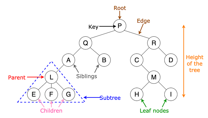
A tree is a data structure composed of a root (at the top) and children nodes. Each child can have only one parent, but multiple children. The nodes at the bottom without children are known as leaf nodes

Recursively, we can define a tree as a root node and zero or more subtrees where each subtree is a tree.

Binary tree
A binary tree is a tree with a condition that:

A parent node can have at most 2 children nodes known as left and right child nodes
Each subtree is a binary tree

Such a tree is used to generate parse trees in SQL

Binary search tree

A binary search tree is used to keep (and lookup values in) a list of sorted numbers. It achieves this by having the properties:

Of a binary tree
All the nodes of the left subtree are less than the root node.
All the nodes of the right subtree are greater than the root node.
Each subtree is a binary search tree

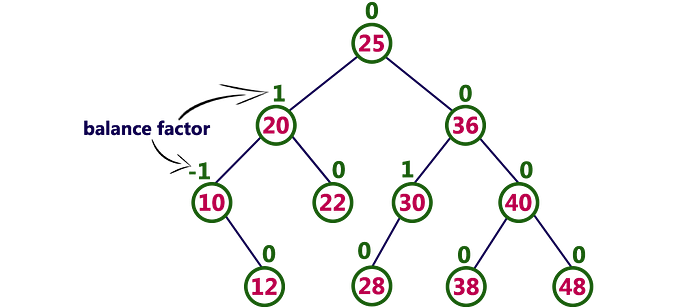
Self-balancing binary search tree (AVL tree)

A balanced binary tree is one where:

For any given node, the difference of the left subtree and right subtree is at most 1
Each subtree is a balanced binary tree

Each node of a self-balancing tree contains a balance factor which is the difference between the left and right subtrees. This value should always be -1, 0, or +1

B-Tree

A B-Tree is a self-balancing binary search tree with key differences:

Each node can have more than one value (at most n-1) and the values are sorted ascending
Each internal node can have more than two children, between n/2 and n. The root has between 2 and n
All the leaf nodes have the same depth i.e. number of edges from the root node

B-Tree by Aexpedito via Wikimedia Commons

n is the order the tree. It’s used to define the number of keys that each node can have. The higher the order the shorter the tree is.

When used to create a database index, each value in a node contains:
a) The key
b) A pointer to the row location
c) Pointers to children nodes

B⁺ Tree

A B⁺ tree has the properties of a B-Tree with the following important differences (when implementing indexes):

All the searchable keys are in the leaf nodes
Only the leaf nodes have pointers to row locations. The internal nodes only have the key and pointers to children nodes
The leaf nodes are doubly linked lists pointing to previous and next sibling nodes. This way, we can traverse back and forth without going back to parent nodes

Linked list

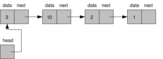
A (singly) linked list is a data structure with nodes stored linearly, similar to an array. However, each node has both a value/data and a pointer to the next node in the list

The last node doesn’t point to anything

This enables us to traverse a list from beginning to end without having to store the list in a single location

Doubly linked list

Similar structure to a (singly) linked list, but each node has another pointer to the previous node

The first node AKA “head” has the previous pointer to nothing.

Enough theory, let’s implement this…

Doubly linked list

To create a doubly linked list, in simple terms, we:

Create nodes of type “DoublyLinkedNode”. The node has value, previous, and next properties
Since we need to use this for our B+ tree index, the value of the node has to be of type “BPlusTreeNode”
Then connect the nodes by defining the previous and next nodes for each node.
The head node has the previous node as None, while the end node has the next node as None.
Define a “DoublyLinkedList” helper class with an attribute head which is the node we’ve already defined.
The class has functions for insert, delete, and traverse operations (See my Github for the full implementation

B+ Tree

This has got to be the most complex data structure I’ve tried to implement! I highly recommend watching this video first, to understand what’s going on in the code

Usage of the tree is split into three parts:

Creating a B+ tree from our data
Converting the leaf nodes of the B+ tree into a doubly-linked list
Using the linkified version of the tree for lookup

The explanation is lengthy. Read it from Github

With the index implemented as a B+ tree, we can query not only for equality conditions like for the hash table

Why B+ Trees to implement indexes:

You need the same number of tree traversals to get the starting point when looking up a value. Remember that all the leaf nodes are at the same level?
With a high enough order of the tree (usually in hundreds) you need a very short tree to store the entire index. This means a relatively smaller space occupied compared to the hash index. The number of traversals to get a value are also lowered
As an inherently ordered data structure, you can do more than equality comparisons as we’ve seen above.
The growth of the tree is more efficient

Downsides of using a B-Tree index:

Insertion and deletion of items is very involved as compared to hash index. I even wasn’t able to implement deletion!
This index may be less performant where the indexed column has a lot of duplicate values. Say we wanted all the value equal to 5:
a) We first traverse from the root of the tree to the leaf node containing 5
b) Since we can’t tell the level of duplication in the index, we need to check any other nodes (forward or backward) that may contain 5. This is easily done since all the leaf nodes are a giant doubly-linked list
c) If there’s a large occurence of 5, we’ll have to check a lot of nodes (O(n)). If the column is highly unique, we’ll stop the traversal of the list very quickly.