Modelling the SIMPLE model of memory

Bayesian cognitive modelling

In this blogpost I am going to use, yet, another example from the book “Bayesian Cognitive Modelling” by Lee & Wagemakers. This book is full of examples in cognitive psychology which can be approached in a Bayesian way. Since the examples are mostly done via WinBUGS, I wanted to see if I can recreate it using brms and stan. So, that is what this blogpost will be about. (I know the book also provides the stan codes, but I want to see how far I can get with brms which has less functionality then base STAN or WinBUGS).

In this example, I will model the SIMPLE model of memory, which measures people’s ability to retain stimuli. The challenge of this model, as you will come to discover, is within its nonlinear curve.

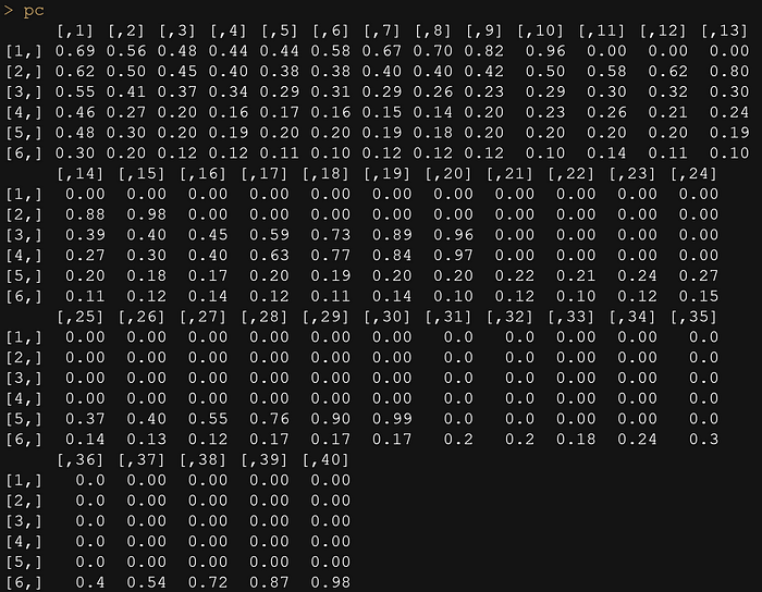
The background is not that important, but what it is the way on how to approach the problem. Let me show you by plotting the data.

But first, load the libraries and the data.

# clears workspace:  
rm(list=ls()) 
library(dplyr)
library(ggplot2)
library(brms)
library(bayesplot)
library(tidybayes)
library(marginaleffects)

y          <- matrix(scan("CaseStudies/Simple/k_M.txt", sep=","), ncol=40, nrow=6, byrow=T) 
n          <- c(1440,1280,1520,1520,1200,1280)
listlength <- c(10,15,20,20,30,40)
pc         <- matrix(scan("CaseStudies/Simple/pc_M.txt", sep=","), ncol=40, nrow=6, byrow=T) 
labs       <- scan("CaseStudies/Simple/labs_M.txt", sep="", what="character")
dsets <- 6 
gsets <- 9

y
pc
labs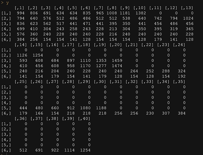

pc<-as.data.frame(t(pc))
colnames(pc)<-labs
d <- pc
Position <- rownames(d)
rownames(d) <- NULL
df <- cbind(Position,d)
str(df)
df_long<-df%>%
  tidyr::pivot_longer(cols=`10-2`:`40-1`,
                      names_to = "Condition",
                      values_to = "PC")
str(df_long)
df_long$Position<-as.numeric(df_long$Position)
df_long<-df_long%>%filter(PC>0)
ggplot(df_long)+
  geom_point(aes(x=Position, 
                 y=PC))+
  theme_bw()+
  facet_wrap(~Condition)

ggplot(df_long)+
  geom_point(aes(x=Position, 
                 y=PC))+
  geom_smooth(aes(x=Position, 
                  y=PC))+
  theme_bw()+
  facet_wrap(~Condition)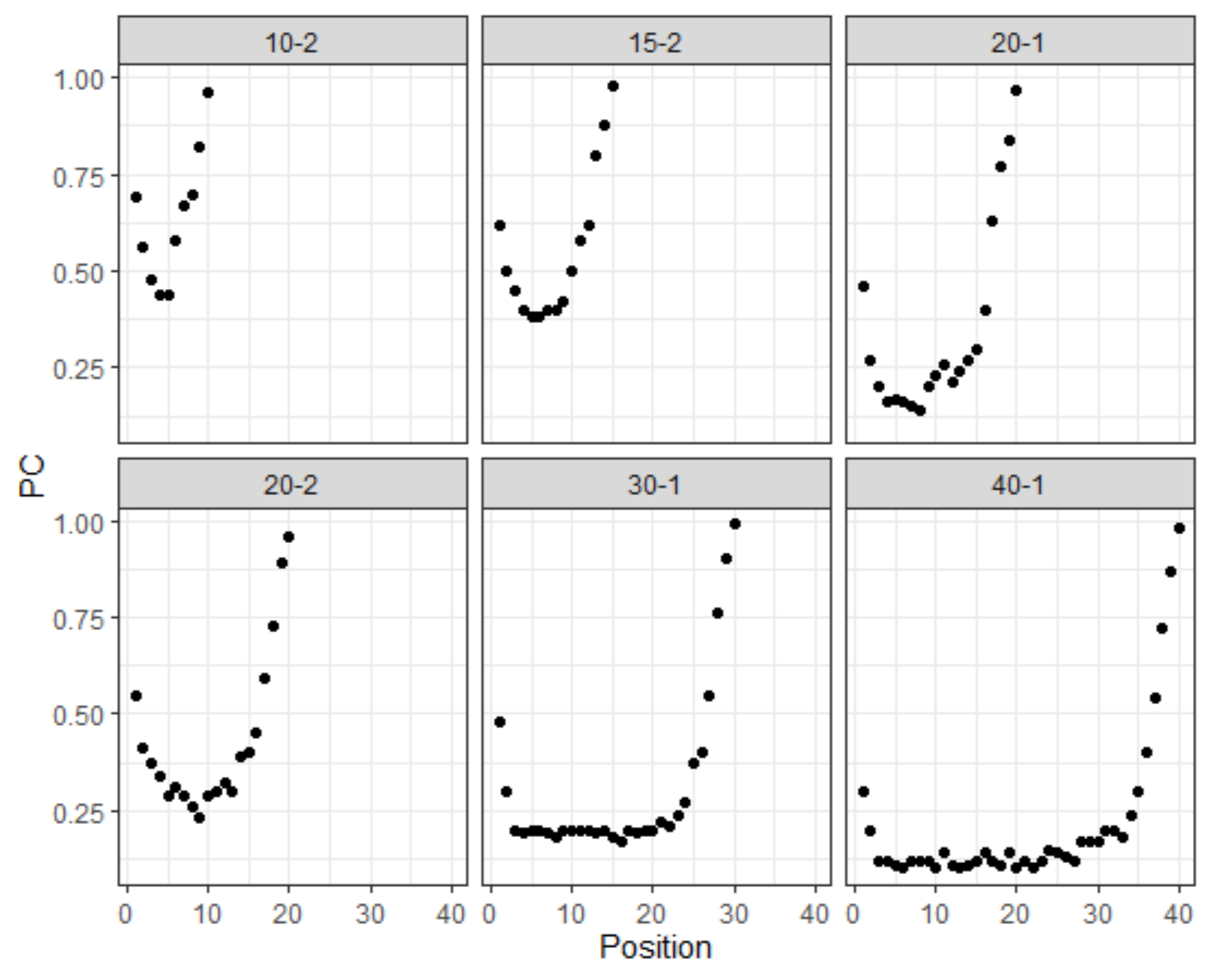

These plot show, for six conditions, the percentage correct in relationship to the position of the stimulus to be retained. It is this patterns that we need to model.

In the book, it is clearly show how complex the model is, also from a cognitive point of view. The models that are then most efficient to use are mechanistic models in which the various parts of the underlying theory are connected to form a model and from which to draw predictions. That model is also what is made in WinBUGS in the book and which can be created using STAN, but I would like to model it using basic brms. Now, this does not mean brms is basic, but I will do a slighlty different model than what is being done in the book. In the end, my job is to model the curve.

I can show the same graph from above using a long format. For that I will need to do some additional transformations.

y<-as.data.frame(t(y))
colnames(y)<-labs
d <- y
Position <- rownames(d)
rownames(d) <- NULL
df <- cbind(Position,d)
str(df)
df_long<-df%>%
  tidyr::pivot_longer(cols=`10-2`:`40-1`,
                      names_to = "Condition",
                      values_to = "Y")
df_long$Position<-as.numeric(df_long$Position)
df_long<-df_long%>%
  arrange(Condition, Position)
df_long$N<-rep(n,each=40)
df_long$PC<-df_long$Y/df_long$N
df_long<-df_long%>%filter(PC>0)
ggplot(df_long)+
  geom_point(aes(x=Position, 
                 y=PC))+
  geom_smooth(aes(x=Position, 
                  y=PC))+
  theme_bw()+
  facet_wrap(~Condition)

And here we have the same plot using a different data frame.

Now, the data is by all means non-linear and there are multiple ways of modelling it. We could use splines, a non-linear function, or we could transform the data and then model it via a more simple solution. Lets try the last suggestion first.

ggplot(df_long)+
  geom_point(aes(x=log10(Position), 
                 y=log10(Y)))+
  geom_smooth(aes(x=log(Position), 
                  y=log10(Y)))+
  theme_bw()+
  facet_wrap(~Condition)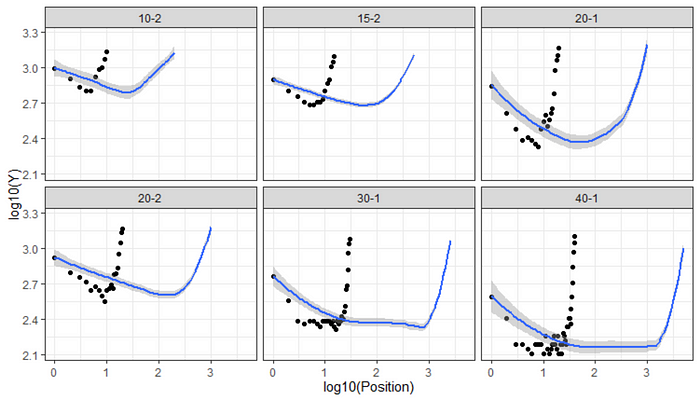

That did not help. At all.

Of to the modelling part. Now, in a previous example I already showed that using the underlying Binomial distribution is a better choice than using the Beta distribution. So lets go for Binomial from the start.

get_prior(Y | trials(N) ~ 
                Position + (1|Condition), 
              data = df_long,
              family=binomial(link = "logit"))
fit<-brms::brm(Y | trials(N) ~ 
                 Position + (1|Condition), 
               data = df_long,
               family=binomial(link = "logit"),
               prior = c(
                 prior(normal(0, 1), class=b, coef=Position ),
                 prior(normal(0, 1), class=Intercept),
                 prior(gamma(1, 1), class=sd, coef=Intercept, group=Condition)), 
               chains=4, 
               cores=6, 
               warmup = 3000,
               iter = 6000)
summary(fit)
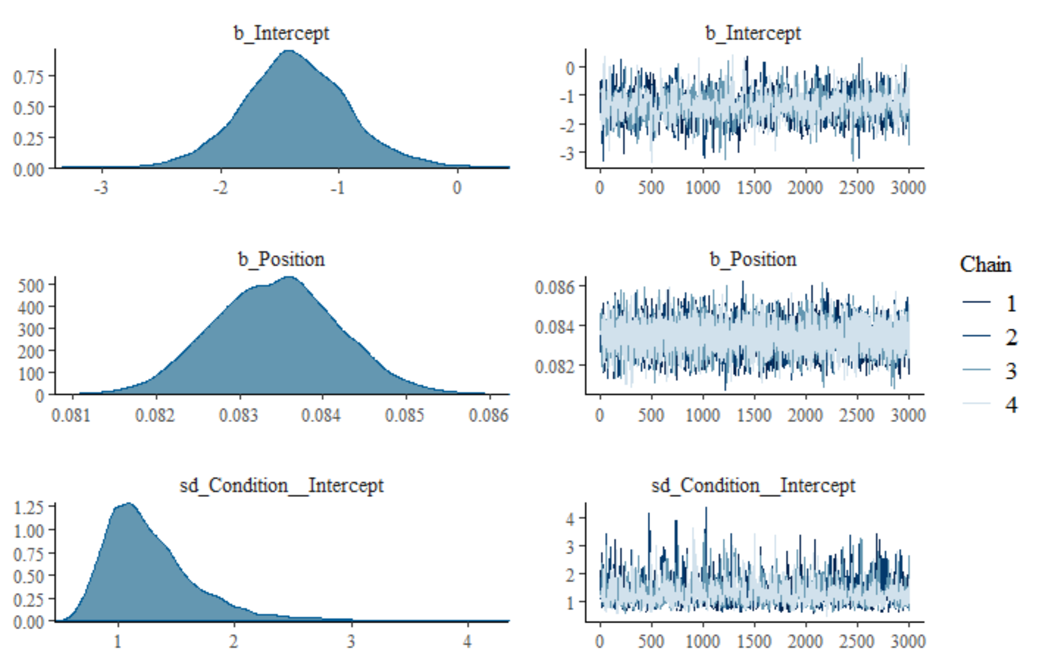
plot(fit)
pp_check(fit, ndraws = 500)
pp_check(fit, type = "error_hist", ndraws = 11)
pp_check(fit, type = "scatter_avg", ndraws = 100)
pp_check(fit, type = "stat_2d")
pp_check(fit, type = "loo_pit")


df_long %>%
  add_epred_draws(fit, 
                  ndraws=100, 
                  allow_new_levels = TRUE) %>%
  ggplot(aes(x = Position, 
             y = Y, 
             group=Condition)) +
  geom_line(aes(y = .epred, group = paste(Condition, .draw)), alpha = 0.25) +
  geom_point(data = df_long, color="black")+
  facet_wrap(~Condition)+
  theme_bw()

Sampling looks good, but the model is not connecting to the data at all. That does not have to be a problem if you are very much convinced that the priors used are suitable.

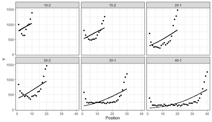
The predictions do not connect to the observations and when you look at the deviations, one would be very hard pressed to maintain that chosen priors and models are sufficient. I would not bet on that.

Another try then, but this time using splines. Splines are very nice way of modelling non-linear patterns, which are still linear in their function. However, the trouble is that a spline often looses part of its interpretation, especially when compared to a non-linear function which is harder to model.

Lets apply the splines in the brms model and see where we end up. The gp part of the spline constitutes a Gaussian Process. Many different types of splines are possible.

fit4<-brms::brm(Y | trials(N) ~ 
                  1 + s(Position, bs="gp") + (1+Position|Condition), 
                data = df_long,
                family=binomial(link = "logit"), 
                chains=4, 
                cores=6, 
                warmup = 3000,
                iter = 6000)

summary(fit4)
pp_check(fit4, ndraws=500)

df_long %>%
  add_epred_draws(fit4, 
                  ndraws=100, 
                  allow_new_levels = TRUE) %>%
  ggplot(aes(x = Position, 
             y = Y, 
             group=Condition)) +
  geom_line(aes(y = .epred, group = paste(Condition, .draw)), alpha = 0.25) +
  geom_point(data = df_long, color="black")+
  facet_wrap(~Condition)+
  theme_bw()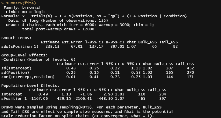

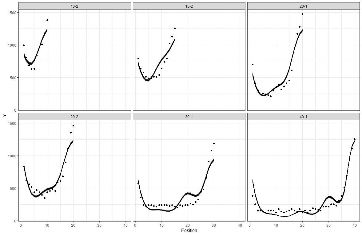
The model has no pre-defined prior (only priors coming from the data itself) which makes it a less stable model. Also, which can be clearly seen, is that the spline does not necessarily know how to deal with the data, which looks like a combination of a power function and an exponential.

Hence, the spline is not the best way to fit the data. There are of course other methods which I will explore now, of which implementing a non-linear function is the best possible way.

Non-linear functions are notorious difficult, so I will start small using a single condition.

df_long_group2<-df_long%>%filter(Condition=="20-1")
plot(df_long_group2$Position, df_long_group2$Y)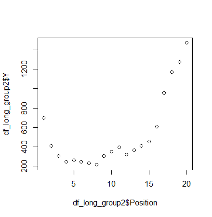

For a single condition I show the position and the number of correct. As you can see this is very much a non-linear function.

Next up I want to apply the non-linear function using the nls program. The formula I am using now is one I found when looking for which to model a parabola. The sinusoidal function should not surprise you as it can model the ups and downs of a cycle, but I wonder if it will find the correct magnitude. Nevertheless, lets get started.

try<-nls(Y ~ b0 + b1*sin(Position)+b2*log(Position), 
         data = df_long_group2,
         start = list(b0 = 100, 
                      b1 = 100,
                      b2 = 100), 
         na.action=na.exclude, 
         control=nls.control(maxiter = 1000, tol = 1e-05))
summary(try)
plot(try)
df_long_group2$pred<-predict(try)
ggplot(df_long_group2)+
  geom_point(aes(x=Position, 
                 y=Y))+
  geom_line(aes(x=Position, 
                y=pred, 
                group=Condition), col="red")+
  theme_bw()

Models fits, but the predictions are off. We see cycles which we should not see.

Even though the model is not good, lets see how the Bayesian model performs using brms. I will apply the same function and part of the priors used in the book as well. These are some ver very uninformative priors. You can hardly call this Bayesian analysis.

fit2<-brms::brm(bf(Y | trials(N) ~ 
                     b0 + b1*sin(Position)+b2*log(Position),
                   b0 + b1 + b2 ~ 1 + (1|Condition), nl=TRUE),
                data= df_long,
                family=binomial(link = "logit"),
                prior = c(
                  prior(uniform(0, 200), class=b, coef=Intercept, nlpar = "b0"),
                  prior(uniform(0, 200), class=b, coef=Intercept, nlpar = "b1"), 
                  prior(uniform(0, 250), class=b, coef=Intercept, nlpar = "b2"),
                  prior(gamma(1, 1), class=sd, group=Condition, nlpar = "b0"),
                  prior(gamma(1, 1), class=sd, group=Condition, nlpar = "b1"),
                  prior(gamma(1, 1), class=sd, group=Condition, nlpar = "b2")), 
                chains=4, 
                cores=6, 
                warmup = 3000,
                iter = 6000)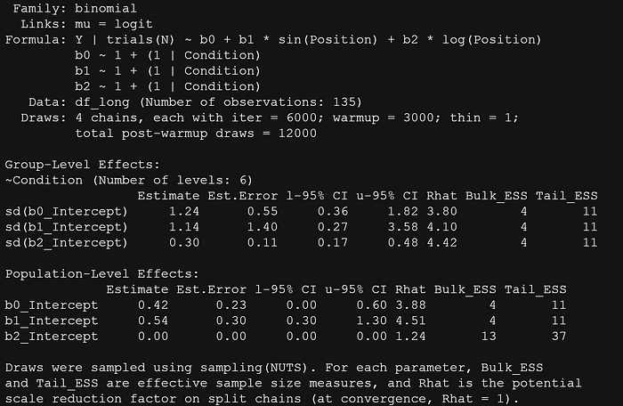

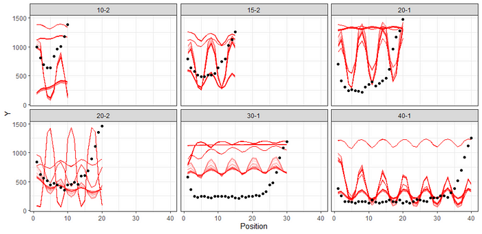
And here we have the output from the model. Just look at the Rhats produced. If you see values such as these, the prediction plots can be a real treat to see. Not because they are correct, but because they will be all over the place.

And yes, they are all over the place!

What will happen if I change the priors? I will now construct uniform priors for the location part and gamma priors for the scale part.

fit3<-brms::brm(bf(Y | trials(N) ~ 
                     b0 + b1*sin(Position)+b2*log(Position),
                   b0 + b1 + b2 ~ 1 + (1|Condition), nl=TRUE),
                data= df_long,
                family=binomial(link = "logit"),
                prior = c(
                  prior(uniform(-10, 10), class=b, coef=Intercept, nlpar = "b0"),
                  prior(uniform(-10, 10), class=b, coef=Intercept, nlpar = "b1"), 
                  prior(uniform(-10, 10), class=b, coef=Intercept, nlpar = "b2"),
                  prior(gamma(1, 1), class=sd, group=Condition, nlpar = "b0"),
                  prior(gamma(1, 1), class=sd, group=Condition, nlpar = "b1"),
                  prior(gamma(1, 1), class=sd, group=Condition, nlpar = "b2")), 
                chains=4, 
                cores=6, 
                warmup = 3000,
                iter = 6000)
summary(fit3)
pp_check(fit3, ndraws=500)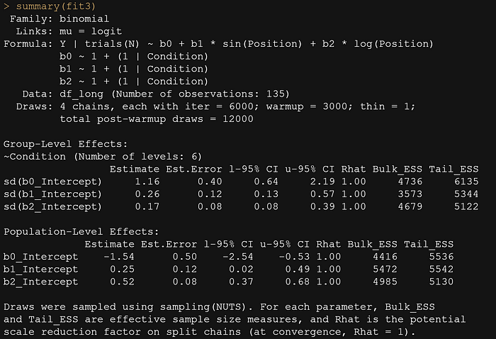

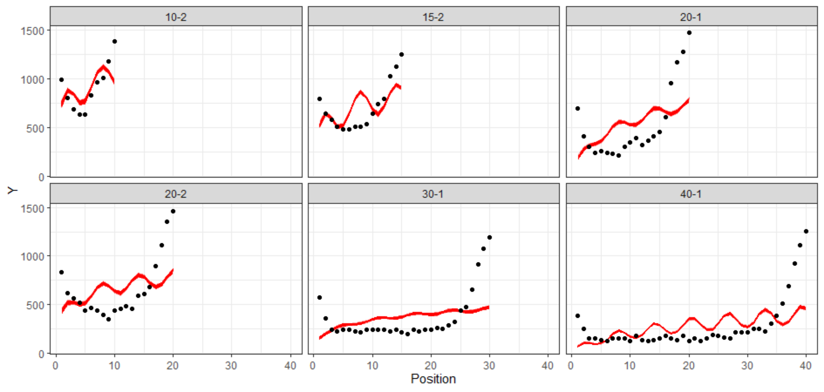
The model looks better as the Rhat values are normal. This means the sampling is stable, but does not mean the model makes sense. However, stable Rhats are a welcome sight.

However, the predictions coming from the model leave much to be desired, behaving very much like a cycle. This should not surprise you, and so it should not surprise you that I will decide that this non-linear function is pretty much useless to model this particular set of observations. Lets move on.

The particular function used in the book is nested, and quite sophisticated. Of course, I could use the STAN code the authors applied, but at this point I do not even want to anymore. I want to see if I can model this pattern in a non-linear way. But before I do that, I want to take one last detour, and that is applying a polynomial function. Very much in line with a spline, it has some easier to interpret output. And its agile. Lets quickly assess.

First, I will test using a linear regression and the lm function.

df_long_group2<-df_long%>%filter(Condition=="20-1")
plot(df_long_group2$Position, df_long_group2$Y)
try<-lm(Y ~ Position + 
          I(Position^2) + 
          I(Position^3), data=df_long_group2)
summary(try)
df_long_group2$pred<-predict(try)
ggplot(df_long_group2)+
  geom_point(aes(x=Position, 
                 y=Y))+
  geom_line(aes(x=Position, 
                y=pred, 
                group=Condition), col="red")+
  theme_bw()

The model and its prediction. Not perfect, but not that bad either.

Now, I will try the same thing using the glm function.

try<-glm(cbind(Y|N) ~ Position + 
          I(Position^2) + 
          I(Position^3), 
         data=df_long_group2, 
         family=binomial)
summary(try)
df_long_group2$pred<-predict(try, df_long_group2, type="link")
ggplot(df_long_group2)+
  geom_point(aes(x=Position, 
                 y=Y))+
  geom_line(aes(x=Position, 
                y=pred, 
                group=Condition), col="red")+
  theme_bw()

Not sure what happened, but something went wrong here. The standard errors are huge and so the fit of the model is not as it should be.

In the end, I do not wish to model the data using a Normal distribution, but with the Binomial. For the priors I will take the normal for the location parameters and gamma for the scale / precision parameter. These are quite wide.

get_prior(bf(Y | trials(N) ~ 
               Position + 
               I(Position^2) + 
               I(Position^3) + 
               (1|Condition)),
          data= df_long,
          family=binomial(link = "logit"))
fit4<-brms::brm(bf(Y | trials(N) ~ 
                     Position + 
                     I(Position^2) + 
                     I(Position^3) +
                   (1|Condition)),
                data= df_long,
                family=binomial(link = "logit"),
                prior = c(
                  prior(normal(200, 50), class=Intercept),
                  prior(normal(0,10), class=b, coef=Position),
                  prior(normal(0,10),  class=b, coef=IPositionE2), 
                  prior(normal(0,10), class=b, coef=IPositionE3),
                  prior(gamma(4, 4), class=sd, group=Condition)), 
                chains=4, 
                cores=6, 
                warmup = 3000,
                iter = 6000)
summary(fit4)
pp_check(fit4, ndraws=500)
df_long %>%
  add_epred_draws(fit4, 
                  ndraws=200, 
                  allow_new_levels = TRUE) %>%
  ggplot(aes(x = Position, 
             y = Y, 
             group=Condition)) +
  geom_line(aes(y = .epred, group = paste(Condition, .draw)), alpha = 0.25, col="red") +
  geom_point(data = df_long, color="black")+
  facet_wrap(~Condition)+
  theme_bw() 

And what I get is another very strange model, nothing I can or should use.

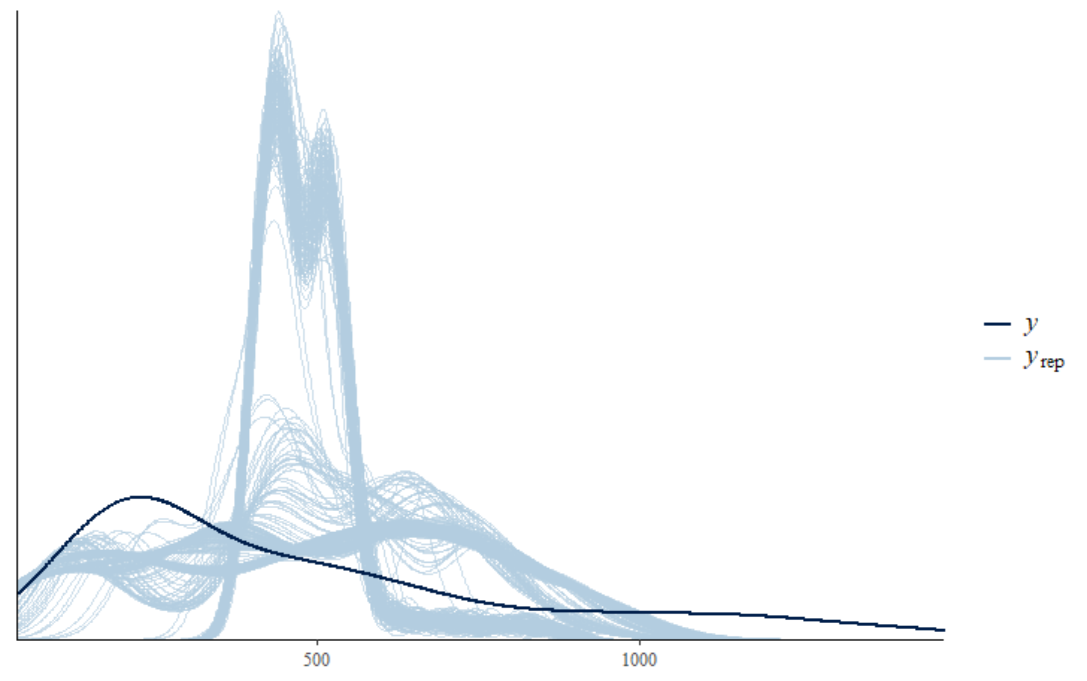
Instead of the polynomial, I could revert back to splines, but this time I will ask the model to make splines per category. This is easily done in brms.

get_prior(bf(Y | trials(N) ~ 
               s(Position, by=Condition)),
          data= df_long,
          family=binomial(link = "logit"))

The priors I need to specify when building a spline for each condition seperately.

For this model, I will stick with uniform priors. Once again, this is weak Bayesian modelling, but I am unsuccessful using polynomials and so I wish to see where the data will bring me.

fit5<-brms::brm(bf(Y | trials(N) ~ 
                     s(Position, by=Condition)),
                data= df_long,
                family=binomial(link = "logit"),
                prior = c(
                  prior(uniform(-10, 10), class=Intercept),
                  prior(uniform(-10, 10), class=b, coef=sPosition:Condition10M2_1),
                  prior(uniform(-10, 10), class=b, coef=sPosition:Condition15M2_1),
                  prior(uniform(-10, 10), class=b, coef=sPosition:Condition20M1_1),
                  prior(uniform(-10, 10), class=b, coef=sPosition:Condition20M2_1),
                  prior(uniform(-10, 10), class=b, coef=sPosition:Condition30M1_1),
                  prior(uniform(-10, 10), class=b, coef=sPosition:Condition40M1_1),
                  prior(gamma(1, 1), class=sds)), 
                chains=4, 
                cores=6, 
                warmup = 3000,
                iter = 6000)
summary(fit5)
pp_check(fit5, ndraws=500)
df_long %>%
  add_epred_draws(fit5, 
                  ndraws=200, 
                  allow_new_levels = TRUE) %>%
  ggplot(aes(x = Position, 
             y = Y, 
             group=Condition)) +
  geom_line(aes(y = .epred, group = paste(Condition, .draw)), alpha = 0.25, col="red") +
  geom_point(data = df_long, color="black")+
  facet_wrap(~Condition)+
  theme_bw()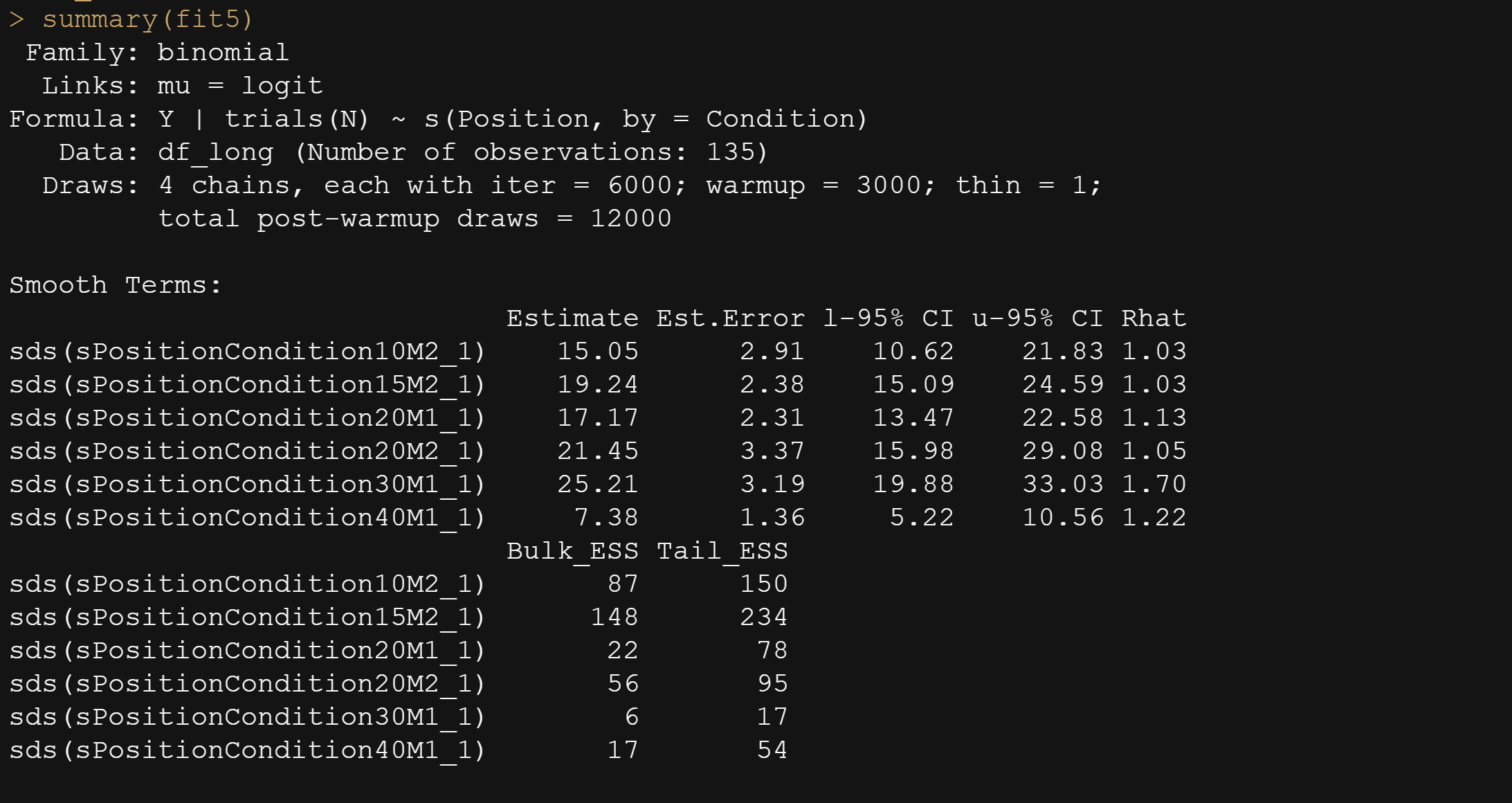

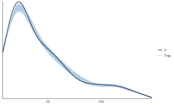
Rhats look better, but certainly not perfect.

Considering the heavy Rhats I would have expected less dense sampling, but this does not look that bad to be honest.

And the prediction, which do not look bad either. Remember, this is full statistical and not mechanical modelling. But in the end, the model does seem to do the trick, at the expense of some loss of information on what the parameters exactly mean.

I am still not satisfied and wish to take a look at a non-linear function one last time. Lets go at it again.

df_long_group2<-df_long%>%filter(Condition=="20-1")
plot(df_long_group2$Position, df_long_group2$Y)
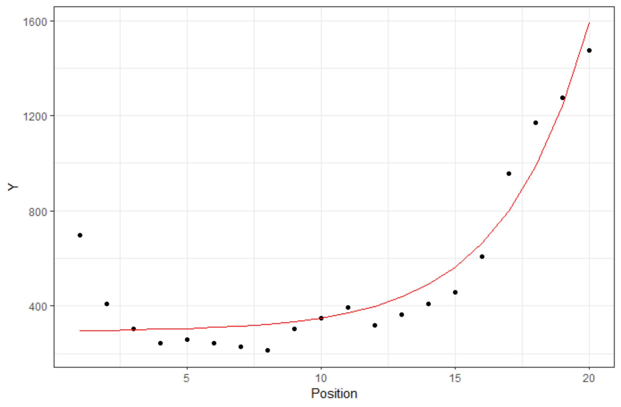
try<-nls(Y ~ a1*exp(b1*Position)+c1, 
         data = df_long_group2,
         start = list(a1 = 1, 
                      b1 = 1,
                      c1 = 1), 
         na.action=na.exclude, 
         control=nls.control(maxiter = 1000, tol = 1e-05))
summary(try)
df_long_group2$pred<-predict(try)
ggplot(df_long_group2)+
  geom_point(aes(x=Position, 
                 y=Y))+
  geom_line(aes(x=Position, 
                y=pred, 
                group=Condition), col="red")+
  theme_bw()

Looks very good. Not perfect, but the best one can expect. However, as you can already see, it cannot deal with the initial descent. This is because the data seem to be a combination of a power function and exponential function. I am sure that a model can be constructed, connecting them both, but that model will mostly likely be just as heavy in the parameters as the spline.

Lets try the same non-linear function on another condition.

df_long_group2<-df_long%>%filter(Condition=="40-1")
plot(df_long_group2$Position, df_long_group2$Y)
try<-nls(Y ~ a1*exp(b1*Position)+c1, 
         data = df_long_group2,
         start = list(a1 = 2, 
                      b1 = 0.5,
                      c1 = 300), 
         na.action=na.exclude, 
         control=nls.control(maxiter = 1000, tol = 1e-05))
summary(try)
df_long_group2$pred<-predict(try)
ggplot(df_long_group2)+
  geom_point(aes(x=Position, 
                 y=Y))+
  geom_line(aes(x=Position, 
                y=pred, 
                group=Condition), col="red")+
  theme_bw()

Also fits, but once again, it will not model the initial descent.

On to the next challenge, which is to place the non-linear function in the Bayesian framework.

get_prior(bf(Y | trials(N) ~ 
               a1*exp(b1*Position)+c1,
             a1 + b1 + c1 ~ 1, nl=TRUE),
          data= df_long,
          family=binomial(link = "logit"))
fit7<-brms::brm(bf(Y | trials(N) ~ 
                     a1*exp(b1*Position)+c1,
                   a1 + b1 + c1 ~ 1, nl=TRUE),
                data= df_long,
                family=binomial(link = "logit"),
                prior = c(
                  prior(uniform(-10, 10), class=b, coef=Intercept, nlpar = "a1"),
                  prior(uniform(-10, 10), class=b, coef=Intercept, nlpar = "b1"), 
                  prior(uniform(-400, 400), class=b, coef=Intercept, nlpar = "c1")), 
                chains=4, 
                cores=6, 
                warmup = 3000,
                iter = 6000)
summary(fit7)
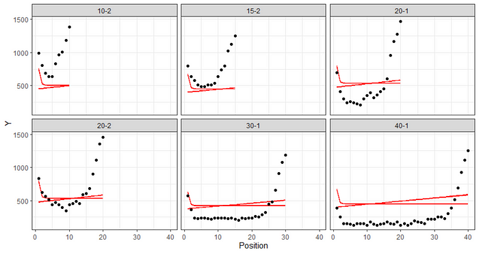
df_long %>%
  add_epred_draws(fit7, 
                  ndraws=100, 
                  allow_new_levels = TRUE) %>%
  ggplot(aes(x = Position, 
             y = Y, 
             group=Condition)) +
  geom_line(aes(y = .epred, group = paste(Condition, .draw)), alpha = 0.25, col="red") +
  geom_point(data = df_long, color="black")+
  facet_wrap(~Condition)+
  theme_bw()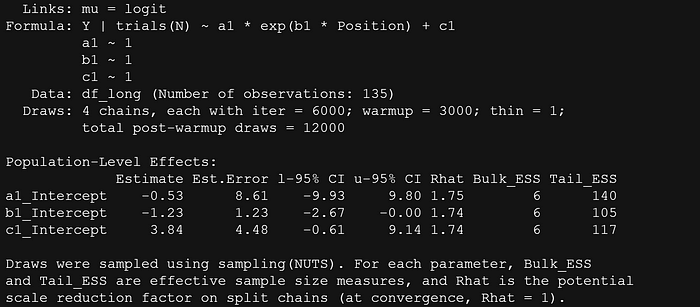       

Sampling is already taking a turn for the worst.

Funny enough, the Bayesian model will try and model the initial descent but then has no parameters left to model the exponential part.

A next try, which will not add much, but I am still doing it, is to build a full non-linear mixed model in which the three parameters are allowed to shift per condition. For the location parameters I am using a uniform prior, and for the scale I am using gamma.

fit7<-brms::brm(bf(Y | trials(N) ~ 
                     a1*exp(b1*Position)+c1,
                   a1 + b1 + c1 ~ 1 + (1|Condition), nl=TRUE),
                data= df_long,
                family=binomial(link = "logit"),
                prior = c(
                  prior(uniform(-10, 10), class=b, coef=Intercept, nlpar = "a1"),
                  prior(uniform(-10, 10), class=b, coef=Intercept, nlpar = "b1"), 
                  prior(uniform(-300, 300), class=b, coef=Intercept, nlpar = "c1"),
                  prior(gamma(1, 1), class=sd, group=Condition, nlpar = "a1"),
                  prior(gamma(1, 1), class=sd, group=Condition, nlpar = "b1"),
                  prior(gamma(1, 1), class=sd, group=Condition, nlpar = "c1")), 
                chains=4, 
                cores=6, 
                warmup = 3000,
                iter = 6000)
summary(fit7)
df_long %>%
  add_epred_draws(fit7, 
                  ndraws=100, 
                  allow_new_levels = TRUE) %>%
  ggplot(aes(x = Position, 
             y = Y, 
             group=Condition)) +
  geom_line(aes(y = .epred, group = paste(Condition, .draw)), alpha = 0.25) +
  geom_point(data = df_long, color="black")+
  facet_wrap(~Condition)+
  theme_bw()

Rhats are even worse and if you look at the predictions it is best to close the graph viewer immediately. This is not helping at all.

Perhaps with some more informative priors, or adding a parameter to the non-linear function I could have improved the model, but for now this is what it is.

In the end, I will stick with the conditional spline model, which builds a spline function per condition. This is not exactly the same model as the one in the book, but it is a model nonetheless.

For my next series, I will look deeper in STAN function itself, which will offer much more versatility.

If anything is amiss, or you just have a comment, let me know!

Mlearning.ai Submission Suggestions