
Everything you need to know about Neural Networks
Courtesy: Kailash Ahirwar (Co-Founder & CTO, Mate Labs)
Intro:
Understanding what Artificial Intelligence is and learning how Machine Learning and Deep Learning power it, are overwhelming experiences. We are a group of self-taught engineers who have gone through that experience and are sharing, our understanding (through blogs) of it and what has helped us along the way, in simplified form, so that anyone who is new to this field can easily start making sense of the technicalities of this technology.
Moreover, during this mission of ours we have created a platform for anyone to be able to build Machine Learning & Deep learning models without writing even a single line of code.

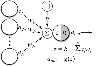
Neuron(Node) — It is the basic unit of a neural network. It gets certain number of inputs and a bias value. When a signal(value) arrives, it gets multiplied by a weight value. If a neuron has 4 inputs, it has 4 weight values which can be adjusted during training time.

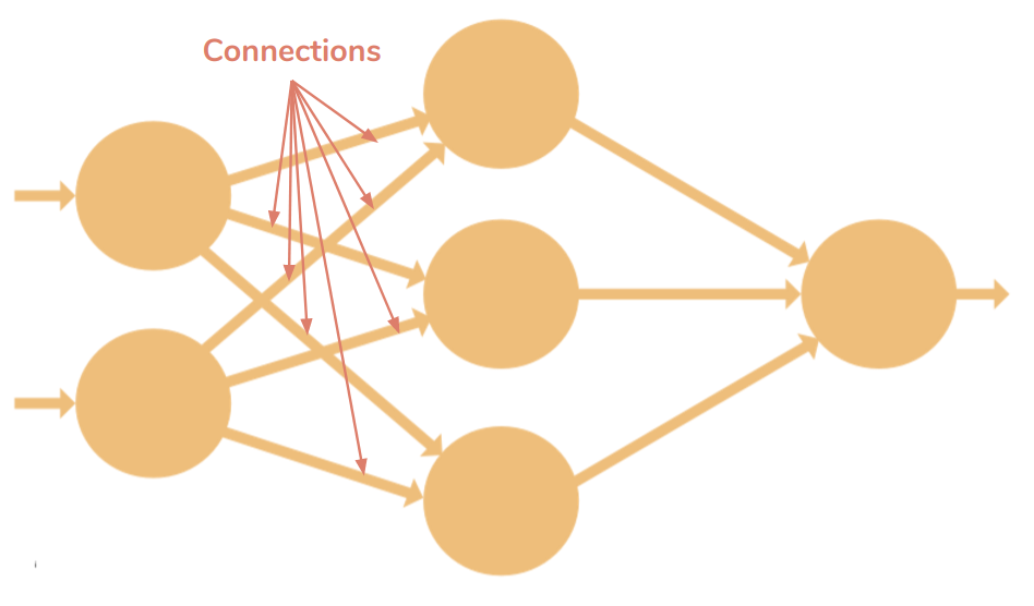
Connections — It connects one neuron in one layer to another neuron in other layer or the same layer. A connection always has a weight value associated with it. Goal of the training is to update this weight value to decrease the loss(error).
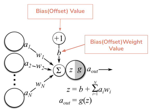
Bias(Offset) — It is an extra input to neurons and it is always 1, and has it’s own connection weight. This makes sure that even when all the inputs are none (all 0’s) there’s gonna be an activation in the neuron.
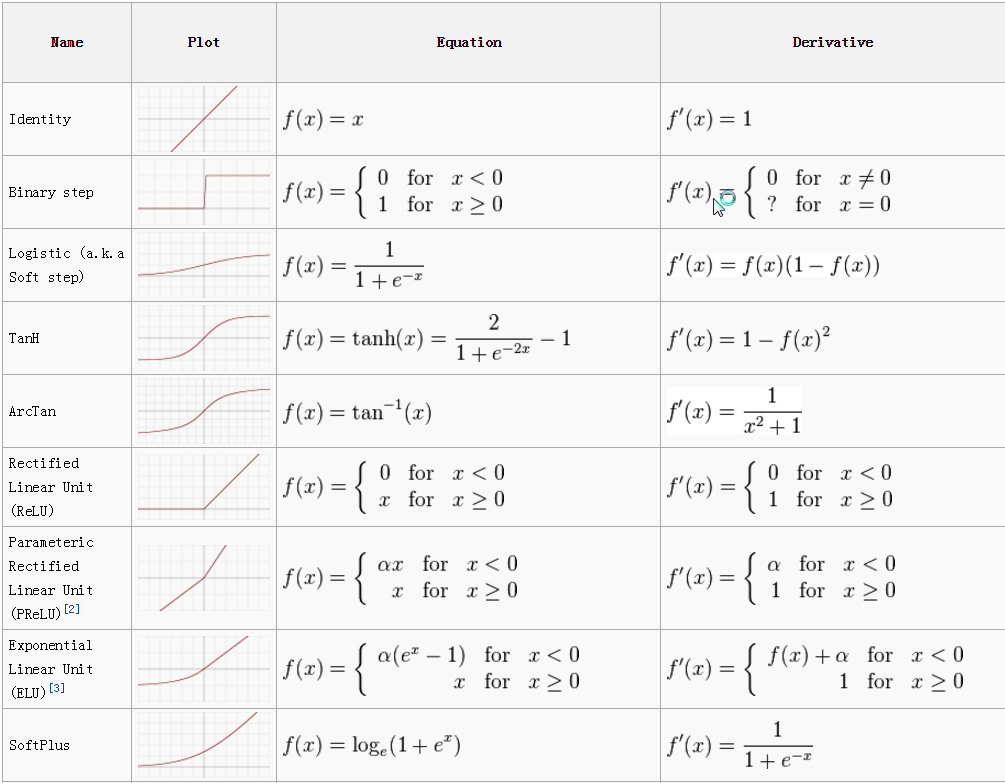
Activation Function(Transfer Function) — Activation functions are used to introduce non-linearity to neural networks. It squashes the values in a smaller range viz. a Sigmoid activation function squashes values between a range 0 to 1. There are many activation functions used in deep learning industry and ReLU, SeLU and TanH are preferred over sigmoid activation function. In this article I have explained the different activation functions available.
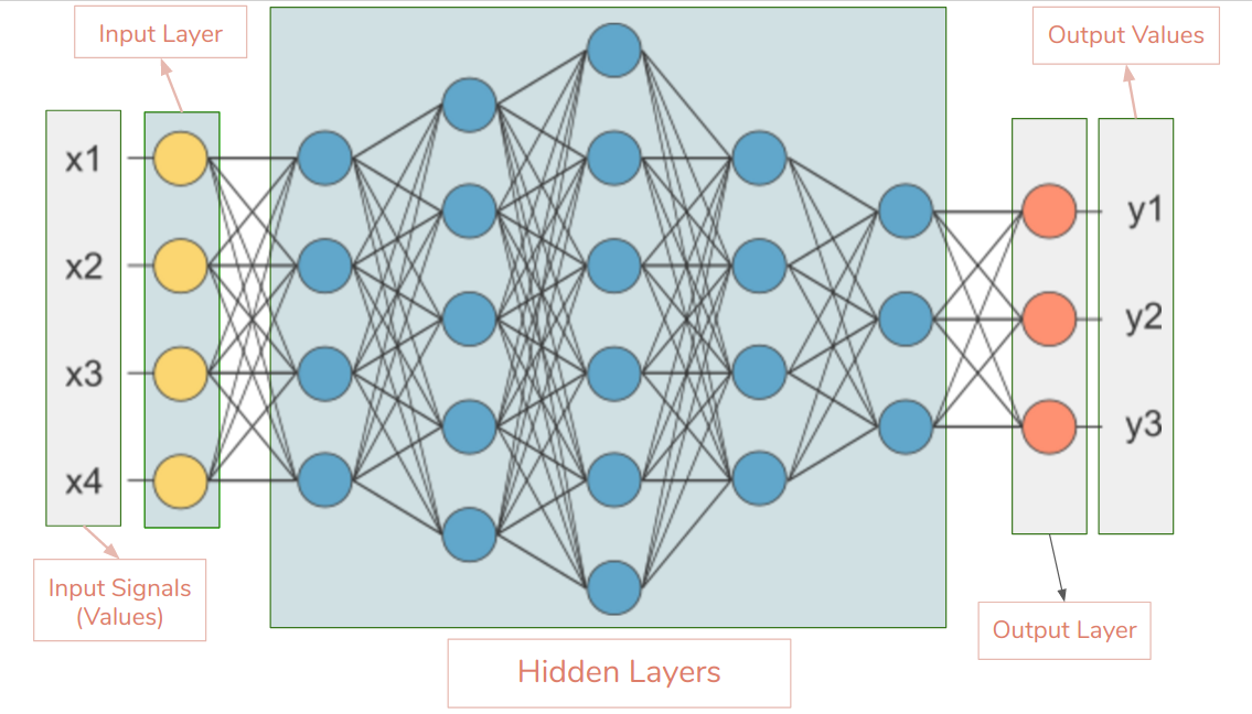
Input Layer — This is the first layer in the neural network. It takes input signals(values) and passes them on to the next layer. It doesn’t apply any operations on the input signals(values) & has no weights and biases values associated. In our network we have 4 input signals x1, x2, x3, x4.
Hidden Layers — Hidden layers have neurons(nodes) which apply different transformations to the input data. One hidden layer is a collection of neurons stacked vertically(Representation). In our image given below we have 5 hidden layers. In our network, first hidden layer has 4 neurons(nodes), 2nd has 5 neurons, 3rd has 6 neurons, 4th has 4 and 5th has 3 neurons. Last hidden layer passes on values to the output layer. All the neurons in a hidden layer are connected to each and every neuron in the next layer, hence we have a fully connected hidden layers.
Output Layer — This layer is the last layer in the network & receives input from the last hidden layer. With this layer we can get desired number of values and in a desired range. In this network we have 3 neurons in the output layer and it outputs y1, y2, y3.
Input Shape — It is the shape of the input matrix we pass to the input layer. Our network’s input layer has 4 neurons and it expects 4 values of 1 sample. Desired input shape for our network is (1, 4, 1) if we feed it one sample at a time. If we feed 100 samples input shape will be (100, 4, 1). Different libraries expect shapes in different formats.
Weights(Parameters) — A weight represent the strength of the connection between units. If the weight from node 1 to node 2 has greater magnitude, it means that neuron 1 has greater influence over neuron 2. A weight brings down the importance of the input value. Weights near zero means changing this input will not change the output. Negative weights mean increasing this input will decrease the output. A weight decides how much influence the input will have on the output.
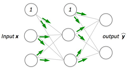
Forward Propagation — Forward propagation is a process of feeding input values to the neural network and getting an output which we call predicted value. Sometimes we refer forward propagation as inference. When we feed the input values to the neural network’s first layer, it goes without any operations. Second layer takes values from first layer and applies multiplication, addition and activation operations and passes this value to the next layer. Same process repeats for subsequent layers and finally we get an output value from the last layer.
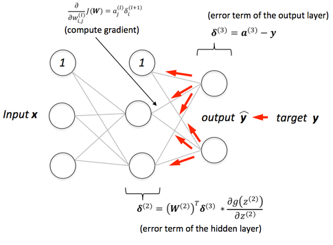
Back-Propagation — After forward propagation we get an output value which is the predicted value. To calculate error we compare the predicted value with the actual output value. We use a loss function (mentioned below) to calculate the error value. Then we calculate the derivative of the error value with respect to each and every weight in the neural network. Back-Propagation uses chain rule of Differential Calculus. In chain rule first we calculate the derivatives of error value with respect to the weight values of the last layer. We call these derivatives, gradients and use these gradient values to calculate the gradients of the second last layer. We repeat this process until we get gradients for each and every weight in our neural network. Then we subtract this gradient value from the weight value to reduce the error value. In this way we move closer (descent) to the Local Minima(means minimum loss).
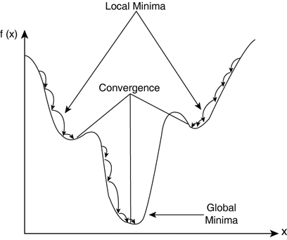
Learning rate — When we train neural networks we usually use Gradient Descent to optimize the weights. At each iteration we use back-propagation to calculate the derivative of the loss function with respect to each weight and subtract it from that weight. Learning rate determines how quickly or how slowly you want to update your weight(parameter) values. Learning rate should be high enough so that it won’t take ages to converge, and it should be low enough so that it finds the local minima.
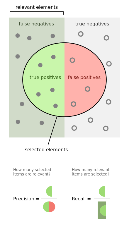
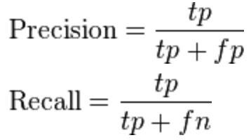
Accuracy — Accuracy refers to the closeness of a measured value to a standard or known value.
Precision — Precision refers to the closeness of two or more measurements to each other. It is the repeatability or reproducibility of the measurement.
Recall(Sensitivity) — Recall refers to the fraction of relevant instances that have been retrieved over the total amount of relevant instances
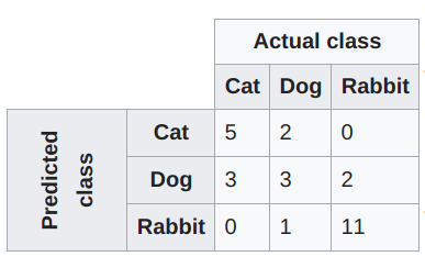
Confusion Matrix — As Wikipedia says:
In the field of machine learning and specifically the problem of statistical classification, a confusion matrix, also known as an error matrix, is a specific table layout that allows visualization of the performance of an algorithm, typically a supervised learning one (in unsupervised learning it is usually called a matching matrix). Each row of the matrix represents the instances in a predicted class while each column represents the instances in an actual class (or vice versa). The name stems from the fact that it makes it easy to see if the system is confusing two classes (i.e. commonly mislabelling one as another).
Convergence — Convergence is when as the iterations proceed the output gets closer and closer to a specific value.
Regularization — It is used to overcome the over-fitting problem. In regularization we penalise our loss term by adding a L1 (LASSO) or an L2(Ridge) norm on the weight vector w (it is the vector of the learned parameters in the given algorithm).
L(Loss function) + λN(w) — here λ is your regularization term and N(w) is L1 or L2 norm
Normalisation — Data normalization is the process of rescaling one or more attributes to the range of 0 to 1. Normalization is a good technique to use when you do not know the distribution of your data or when you know the distribution is not Gaussian (a bell curve). It is good to speed up the learning process.
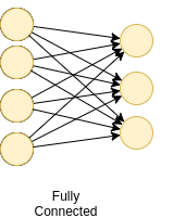
Fully Connected Layers — When activations of all nodes in one layer goes to each and every node in the next layer. When all the nodes in the Lth layer connect to all the nodes in the (L+1)th layer we call these layers fully connected layers.
Loss Function/Cost Function — The loss function computes the error for a single training example. The cost function is the average of the loss functions of the entire training set.
- ‘mse’: for mean squared error.
- ‘binary_crossentropy’: for binary logarithmic loss (logloss).
- ‘categorical_crossentropy’: for multi-class logarithmic loss (logloss).
Model Optimizers — The optimizer is a search technique, which is used to update weights in the model.
- SGD: Stochastic Gradient Descent, with support for momentum.
- RMSprop: Adaptive learning rate optimization method proposed by Geoff Hinton.
- Adam: Adaptive Moment Estimation (Adam) that also uses adaptive learning rates.
Performance Metrics — Performance metrics are used to measure the performance of the neural network. Accuracy, loss, validation accuracy, validation loss, mean absolute error, precision, recall and f1 score are some performance metrics.
Batch Size — The number of training examples in one forward/backward pass. The higher the batch size, the more memory space you’ll need.
Training Epochs — It is the number of times that the model is exposed to the training dataset.
One epoch = one forward pass and one backward pass of all the training examples.

About
At Mate Labs we have built Mateverse, a Machine Learning Platform, where you can build customized ML models in minutes without writing a single line of code. Our platform enables everyone to easily build and train Machine Learning models, without writing a single line of code.
Let’s join hands.
Share your thoughts with us on Twitter.
Tell us if you have some new suggestion. Our ears and eyes are always open for something really exciting.

