ForeCGAT: Predicting diagnosis from genetic assays

Matt Macellaio, an Insight Health Data fellow in Fall 2017, is completing his Ph.D. in neurobiology at the University of Chicago. There, he studied the precision of single neurons in visual cortex and simulated neural population responses to test competing population decoding algorithms.

This fall, I spent time at Insight Data Science consulting with a company that analyzes genetic data. By applying specifically chosen algorithms and analytical tools to genetic and diagnostic data, I was able to show that genetic risk factors can be gleaned from an example dataset and used to predict susceptibility to some conditions that are not typically assumed to have strong genetic underpinnings at first glance, or which are affected by multi-gene interactions.

Background

Nearly every time I look up lately, I see a new article about the genetic data revolution or an academic paper discovering genes linked to a deadly disease. Fifteen years after the official completion of the Human Genome Project, our world has been permanently shaped by its impacts, primarily by sparking the creation of myriad biochemical and bioinformatics tools. Now, companies and private citizens alike wrestle with the question of how best to use this most personal of data to potentially improve our health and that of others who may share similar genetic variants.

Genome-wide association studies (GWAS) have significantly contributed to our knowledge of gene-disease connections. These studies compare the likelihood of mutations across the genome in people diagnosed with a disease to the likelihood of those mutations in healthy people. Genetic variants that show significantly altered likelihood between the groups can then be highlighted as putative disease markers or causes, and can lead to clinical trials for drug targets or genetic assays. These targeted variants typically fall into two main categories: single-nucleotide polymorphisms (SNPs, mutations at a single base defined either by the existence of any mutation or the specific base change) or copy-number variations (CNV, repeats or deletions of a portion of the genome, defined by the number of copies). However, these studies require numerous (>1000) patients and are necessarily large, as they may query bases across the entire genome.

Disease-relevant SNPs can now be targeted with assays and be used to clarify the risk that people have for certain diseases, and medical groups or insurance companies with access to genetic data would like to use such assay data to help doctors improve diagnoses or target medications. Here, I use targeted genetic assay data to train a machine-learning model in Python to potentially improve medical outcomes for patients with a range of diagnoses, regardless of whether their diagnosis is commonly regarded as having a strong genetic component.

Data Exploration

The company I consulted for works with individual research labs to provide clinical diagnostics and data management solutions. They provided me with two kinds of data from 3000 patients: their diagnosis as an ICD-10 code, and their results for a number of genetic assays (Figure 1). The assays included data on SNPs — either the bases observed by the assay (A/A, A/G); the mutation present (T>C if the typical base is T but C was observed); whether a specific SNP was present; or CNVs (Figure 2).

Figure 1. Raw dataset: black indicates that a specific genetic test was performed on a patient’s sample.

Figure 2. Some types of data present, as shown by a reduced dataset.

I had an interestingly complicated dataset: many of the conditions these patients had been diagnosed with are complex diseases, and are not easily reducible to specific genes or mutations. The categories with the most patients are shown in Figure 3, and range from conditions like hypertension with genetic and behavioral roots, to STI-related conditions for which we would not expect to see genetic underpinnings. Therefore, I focused on diagnosis codes with more than 50 patients diagnosed to maximize the distribution of data I observed and the conclusions I could draw from them.

Figure 3. Diagnosis codes with over 100 patients: of these, the codes I used for later analysis are indicated in red.

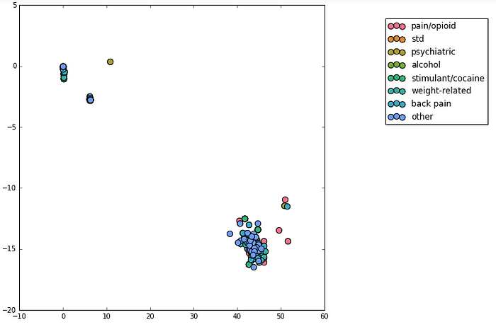
In an attempt to increase the power of my tools, I manually grouped these most prevalent diagnostic codes into 7 main categories: those related to pain/opioid medication, to STDs, to psychiatric issues (e.g. depression), stimulant and cocaine dependence/abuse, weight-related issues (e.g. hypertension and hyperlipidemia), back pain, and alcohol abuse. All others were combined into another bin. My hope was that I could reduce the dimensionality of the genetic data and discover some larger trends. First, I relabeled the genetic results categorically: each different result from a test received a different number (e.g. ‘A/A’ might become ‘1’, ‘A/G’ became ‘2’), and samples with no test performed were labeled with ‘0'. I performed two dimensionality reduction techniques, truncated SVD (Figure 4) and t-SNE, and found that the main clusters appeared to separate based on which tests were performed, not on the results of those tests.

Figure 4. Truncated SVD of dataset, grouped by rough diagnosis category.

Not all patients had all assays performed, and very few assays had data from more than 250 patients, so I had to balance the amount of data I could use with the number of samples I had per test. I chose to focus on a cluster of 105 tests and 1822 patients, still resulting in data for over 220 patients per test. Also, instead of the numerical categorization of assay results, I used one hot encoding, where each result becomes its own feature, and each sample takes on a binary value of whether it exhibits that result, as visualized in Figure 5.

Figure 5. One hot encoded genetic assay data, where black indicates a value of 1.

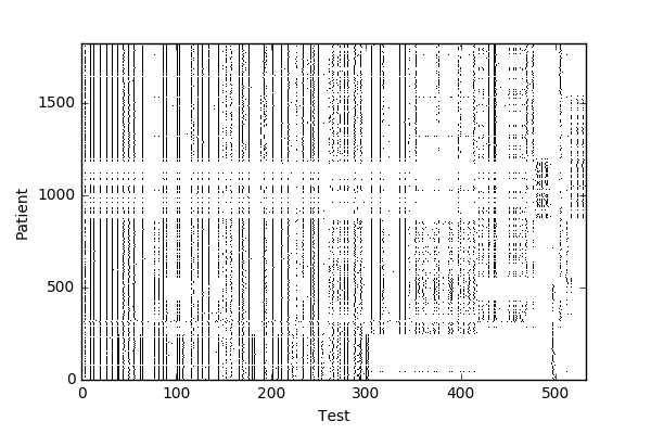
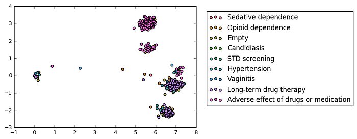
One hot encoding was also a necessary transformation for the data, since the categories did not easily map onto numerical values that would be useful in a regression, for example. I checked again after this whether a reduced dataset would cluster, but to no avail (Figure 6).

Figure 6. Truncated SVD on the reduced, one hot encoded dataset showed no helpful clusters.

Model Training and Results

To uncover patterns in the data that could allow me to predict diagnosis, I trained logistic regression models using scikit-learn separately on each of 22 diagnosis categories. Because of the sparsity of my data, I chose to use lasso regularization, the primary benefit of which is to reduce the weight of any features that don’t contribute to the model to 0. In addition, I had to take into account the imbalanced data: the number of diagnosed patients for each model ranged from 50 to 274, compared to the total sample of 1822 patients. Training a regression model without balancing the diagnosed/undiagnosed classes would allow the model to predict the larger-represented class and still pick correctly most of the time. After trying both undersampling by matching the size of the undiagnosed class to that of the diagnosed one, and oversampling by choosing samples from the diagnosed class with replacement to match the size of the undiagnosed class, I oversampled to have as much variety in each class as possible. Models were trained using 80% of each class before oversampling, and tested on the remaining 20%. I ran 100 resampling loops per diagnosis, training the model and computing the ROC on each loop to negate any results that were potentially due to the small sample size.

Models for 9 diagnoses had an AUC above 0.6, and models for 6 of those had an AUC above 0.7. A key part of the logistic regression model that led to me choosing it was that I could observe the weights contributing to the model, explore what genes and mutations corresponded to those important features, and potentially validate the model by verifying that those genes would make sense to be weighted heavily.

One example model is that trained on the “Adverse effects of drugs or medication” (ICD-10 code T50.905A). The model resulted in an AUC of 0.75, with a few features exhibiting weights with magnitudes greater than 0.10 (Figure 7). Positive weights suggest that the model is using mutations that are positively correlated with, or potentially causative of, diagnosis of this condition; negative weights could indicate mutations that are negatively correlated with, or protective variants against, this condition.

Figure 7. Logistic regression suggests many factors impacting the effect of medications

The top-weighted SNP is rs7900194, a thymine (T) to guanine (G) mutation in the CYP2C9 gene which codes for one of the key liver metabolic enzymes of the cytochrome P450 class. Mutations in this enzyme are associated with alterations in the metabolism of coumadin, a commonly-used blood thinner. Metabolism changes could conceivably change the expected decrease over time in the plasma concentration of coumadin to the point that it would negatively affect a patient.

In comparison, the second most highly weighted SNP is rs55817950 (G/G), the most common variant of a base in another cytochrome P450 family enzyme, CYP3A5. The mutation to A renders the enzyme nonfunctional, and interferes with the metabolism of a number of medications. Therefore, a functional version of the enzyme could be a protective factor against this diagnosis.

Figure 8. Similarities between important features in diagnoses of drug dependence.

Another group of models was those attempting to predict opioid dependence, stimulant dependence, and sedative dependence (AUC = 0.8, 0.78, and 0.76, respectively, Figure 8). All three models pointed to mutations in the CYP2D6 gene as a predictive feature. Importantly, CYP2D6 is a cog in a number of critical drug-related and addiction-related pathways. It metabolizes opioids into morphine, and also breaks down stimulants such as methamphetamine into further psychoactive compounds. In addition, it has a minor role in the biosynthesis of dopamine, a neurotransmitter that is widely implicated in the development of addiction and dependence-related behaviors. Therefore, mutations to this gene could potentially have a link to any or all of these conditions.

Finally, an interesting test case is one diagnosis category that was unlabeled (denoted [Empty] above, Figure 9). One of the strongest weights the model used to predict this diagnosis was an assay targeting SNPs in two locations on the APOE gene where thymine bases mutated to cytosine. The variant, termed ApoE4, is associated with the onset of Alzheimer’s disease, suggesting that this diagnosis could be related to dementia or Alzheimer’s.

Figure 9. Genetic data points to unknown diagnosis potentially being Alzheimer’s or dementia.

Conclusions and Future Directions

My modeling of complex disease risk raises some questions. Chief among these is how well the models and predictions based on this sample and these assays will apply more widely to a larger population and allow for diagnostic power. Due to the restricted size of these samples, I suggest caution while interpreting my results, especially their extension to early diagnosis of conditions. Since susceptibility to addictive behavior necessarily predates clinical levels of substance dependence, any genetics underpinning dependence may be more predictive of the likelihood of conversion from the former state to the latter, than of the likelihood of substance use itself. With a larger patient sample, an ideal next step would be to apply a classification algorithm, since classification more closely matches the real-life problem of picking a single diagnosis from many possibilities.

Demo slides available here