Generative Adversarial Networks — Simply Explained

Adversarial Training
- Adversarial training in machine learning can be traced back to research on vulnerabilities in email spam filters around the early 2000s. Researchers observed that the ML models used for spam filtering could be tricked by manipulating the input data. E.g., spammers would add specific words to their emails to bypass filters.
- Around 2013, the term “adversarial examples” was coined, highlighting how small, imperceptible changes in input data could cause ML models to make mistakes.
- These findings ultimately led to the development of adversarial training techniques. By exposing models to adversarial examples during training, researchers could improve their robustness and make them less susceptible to real-world attacks.
Adversarial Nets
- In 2014, Ian Goodfellow et al. introduced a deep learning architecture known as Adversarial Nets (more generally know as Generative Adversarial Networks (GANs)) that uses adversarial training. The GAN architecture includes two deep neural network models — a generator and a discriminator. This architecture corresponds to a two-player min-max game, where the generator and the discriminator are two adversary players, discriminator tries to maximize the probability of correctly classifying data generated by the generator as fake and at the same time, the generator tries to minimize the probability of discriminator correctly classifying its output as fake.
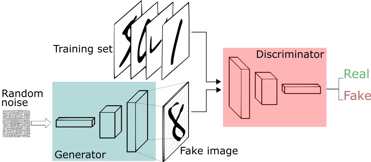
- The generator generates datasamples from a random probability distributionn and passes it to the discriminator for classifying as fake or real. The discriminator’s task is to identify this generated data as fake i.e., the discriminator learns to determine whether the data is from the generator’s distribution or the real data distribution.

In Figure 1 (d) above, we can see that the real and the learned data distributions are overlapping and indistinguishable.
- The generator wants the discriminator to be fooled as much as possible. It aims to minimize the discriminator’s ability to correctly classify real vs. fake data. The discriminator wants to maximize its ability to distinguish real data from generated data. The competition between the generator and the discriminator drives both the models to improve their methods until the generated data is indistinguishable from the real data.
- The generator model is typically a multilayer perceptron and the discriminator model is typically a convolutional neural network that tries to classify fake and real data samples.
- Initially, the generator knows nothing about the real data distribution and the discriminator does not know the difference between the real and fake data. So the discriminator receives two different types of data batches — one of real data samples from the training data and other of noisy samples.
- As training continues, generator learns the data distribution of the training dataset and its ability to create data resembling the training data improves, simultaneously the discriminator’s ability to identify fake data improves. Finally, the generator’s sample becomes indistinguishable from training data.
- Here is the extract from the original GAN paper:
“The GAN architecture includes two models which are trained simultaneously- a generative model G that captures the data distribution, and a discriminative model D that estimates the probability that a sample came from the training data rather than G. The training procedure for G is to maximize the probability of D making a mistake…. This adversarial training approach pushes the generator to create ever-more realistic outputs”
Here is the original training algorithm as per the paper:

Loss function for GAN
- In the GAN architecture, the discriminator receives data from the real training dataset as well as the data generated by the generator.
- The discriminator needs to output probabilities near 1 for real data and near 0 for fake data. Total loss of the discriminator is sum of two partial losses — loss for maximizing the probabilities for the real data samples and the loss for minimizing the probability of fake samples.
- GAN also needs two optimizers one each for the discriminator and the generator.
- The GAN architecture introduced in the Ian Goodfellow paper (Adversary Nets), use a loss function known as min-max loss:

Here D(x) is the probability that data sample x is from real training data. Discriminator is trained to maximize probability of correctly classifying fake and real data samples. [1-D(G(z))] is the probability that discriminator classifies the sample generated by the generator G(z) as fake.
Let us code a GAN from scratch:
We will use keras for building the model and train it on MNIST dataset.
#imports
import numpy as np
import matplotlib.pyplot as plt
import keras
from keras.models import Model, Sequential
from keras.datasets import mnist
from keras import layers
from keras.layers import Activation, Dense, Dropout, Input, LeakyReLU
# Load MNIST dataset, it contains 70000 images of resolution 28*28
# train_images contain 60000 images and test_images contain 10000 images
(train_images, _), (_, _) = keras.datasets.mnist.load_data()
# Normalize pixel values to be between -1 and 1
train_images = (train_images.astype(np.float32) - 127.5) / 127.5
# Reshape and expand dimensions
train_images = train_images.reshape(train_images.shape[0], 28, 28, 1)Set up the parameters for your GAN models
# Set up GAN parameters
latent_dim = 100
# Generator model contains dense layer, two blocks of Conv2d, BN and LeakyReLu layers
# and a final Conv2d layer
generator = keras.Sequential([
    layers.Input(shape=(latent_dim,)),
    layers.Dense(7 * 7 * 128),
    layers.Reshape((7, 7, 128)),
    layers.Conv2DTranspose(128, (4, 4), strides=(2, 2), padding='same'),
    layers.BatchNormalization(),
    layers.LeakyReLU(alpha=0.01),
    layers.Conv2DTranspose(128, (4, 4), strides=(2, 2), padding='same'),
    layers.BatchNormalization(),
    layers.LeakyReLU(alpha=0.01),
    layers.Conv2D(1, (7, 7), activation='tanh', padding='same')
])

# Discriminator model
discriminator = keras.Sequential([
    layers.Input(shape=(28, 28, 1)),
    layers.Conv2D(64, (3, 3), strides=(2, 2), padding='same'),
    layers.LeakyReLU(alpha=0.01),
    layers.Conv2D(128, (3, 3), strides=(2, 2), padding='same'),
    layers.LeakyReLU(alpha=0.01),
    layers.GlobalMaxPooling2D(),
    layers.Dense(1, activation='sigmoid')
])
# Compile discriminator
discriminator.compile(optimizer=keras.optimizers.Adam(learning_rate=0.001, beta_1=0.5),
                      loss='binary_crossentropy', metrics=['accuracy'])
# Make the discriminator non-trainable when combined with the generator
discriminator.trainable = False
# Combined GAN model
gan_input = keras.Input(shape=(latent_dim,))
generated_image = generator(gan_input)
gan_output = discriminator(generated_image)
gan = keras.Model(gan_input, gan_output)
gan.compile(optimizer=keras.optimizers.Adam(learning_rate=0.0002, beta_1=0.5),
            loss='binary_crossentropy')
Let us now train our GAN and plot the generated images after every 5 epochs.
# Training loop
epochs = 100
batch_size = 64
for epoch in range(epochs):
    # Generate random noise as input for the generator
    noise = np.random.normal(0, 1, size=(batch_size, latent_dim))
    # Generate fake images with the generator
    generated_images = generator.predict(noise)
    # Select a random batch of real images from the MNIST dataset
    idx = np.random.randint(0, train_images.shape[0], batch_size)
    real_images = train_images[idx]
    # Combine real and fake images into a single batch
    X = np.concatenate([real_images, generated_images])
    # Labels for real and fake examples
    y_dis = np.zeros(2 * batch_size)
    y_dis[:batch_size] = 0.9  # Label smoothing for real images
    # Train the discriminator
    d_loss = discriminator.train_on_batch(X, y_dis)
    # Generate new random noise for the generator
    noise = np.random.normal(0, 1, size=(batch_size, latent_dim))
    # Labels for generated images (pretend they are all real)
    y_gen = np.ones(batch_size)
    # Train the generator
    g_loss = gan.train_on_batch(noise, y_gen)
    # Print progress and save generated images at specified intervals
    if epoch % 5 == 0:
        print(f"Epoch {epoch}, D Loss: {d_loss[0]}, G Loss: {g_loss}")
        # Save generated images
        generated_images = generated_images * 0.5 + 0.5  # Rescale to 0-1
        fig, axs = plt.subplots(8, 8, figsize=(12, 12))
        cnt = 0
        for i in range(8):
            for j in range(8):
                axs[i, j].imshow(generated_images[cnt, :, :, 0], cmap='gray')
                axs[i, j].axis('off')
                cnt += 1
        plt.show()
References:
1. Generative Adversarial Networks, Ian J. Goodfellow, Jean Pouget-Abadie, Mehdi Mirza, Bing Xu, David Warde-Farley, Sherjil Ozair, Aaron Courville, Yoshua Bengio, arXiv:1406.2661v1.
2. A Short Introduction to Generative Adversarial Networks, Thalles Santos Silva, https://sthalles.github.io/intro-to-gans/
4. https://medium.datadriveninvestor.com/generative-adversarial-network-gan-using-keras-ce1c05cfdfd3