Transfer Learning Using Feature Extraction In Deep Learning

In this blog, we will see the example of transfer learning using feature extraction. We will take the convolutional base of a previously-trained network for new data set, then we will training a new classified on top of the ouput. In this blog we will use VGG16 pre-trained model as convolution base.

What is Transfer Learning?

Normally, very few people train an entire Convolutional Network from scratch, because we don’t have sufficient dataset size.

Transfer learning is a method for feature representation from a pre-trained model that we don’t need to train a new model from scratch. A pre-trained network is simply a saved network previously trained on a huge dataset, typically on a large-scale image classification task. We can use pre-trained model, which is trained on ImageNet(ImageNet, which contains 1.2 million images with 1000 categories). ImageNet contains many animal classes, including different species of cats and dogs. The weights obtained from the models can be reused in other computer vision tasks.

There ate two main Transfer Learning methods are:

Feature extraction

In feature extraction, we take a ConvNet pretrained on ImageNet, remove the last fully-connected layer (this layer’s outputs are the 1000 class scores for a different task like ImageNet), then treat the rest of the ConvNet as a fixed feature extractor for the new dataset. These features are then run through a new classifier, which is trained from scratch.

It is called feature extraction because we use the pre-trained CNN as a fixed feature-extractor, and only change the output layer.

Created by Nutan

Fine-tuning

The fine-tuning strategy is to not only replace and retrain the classifier on top of the ConvNet on the new dataset, but to also fine-tune the weights of the pretrained network by continuing the backpropagation.

In this blog we will use VGG16 pre-trained model as convolution base. So first learn more about VGG16.

What is VGG16?

VGG16 Architecture

Source

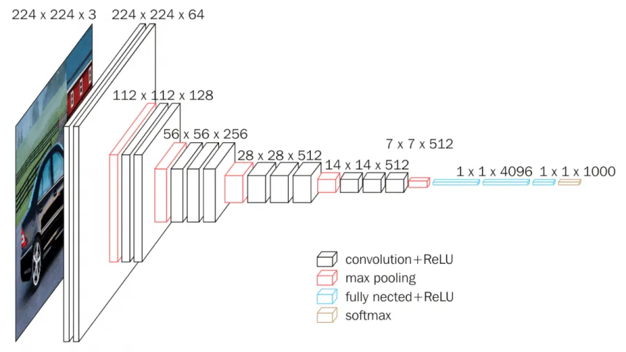
We are using VGG16 as convolution base network, which is trained on ImageNet, then we will add new classifier on top of these features.

Instantiate the VGG16 model:

The VGG16 model, among others, comes pre-packaged with Keras. We can import it from the keras.applications module.

Note: each Keras Application expects a specific kind of input preprocessing. For VGG16, call tf.keras.applications.vgg16.preprocess_input on your inputs before passing them to the model.

`vgg16.preprocess_input` will convert the input images from RGB to BGR,
then will zero-center each color channel with respect to the ImageNet dataset, without scaling.

VGG16(include_top=True, weights=’imagenet’, input_tensor=None, input_shape=None, pooling=None, classes=1000, classifier_activation=’softmax’)

Args:
include_top: whether to include the 3 fully-connected layers at the top of the network.

weights: one of `None` (random initialization), ‘imagenet’ (pre-training on ImageNet), or the path to the weights file to be loaded.

input_tensor: optional Keras tensor (i.e. output of `layers.Input()`) to use as image input for the model.

input_shape: optional shape tuple, only to be specified
if `include_top` is False (otherwise the input shape has to be `(224, 224, 3)` (with `channels_last` data format) or `(3, 224, 224)` (with `channels_first` data format). It should have exactly 3 input channels, and width and height should be no smaller than 32. E.g. `(200, 200, 3)` would be one valid value.

pooling: Optional pooling mode for feature extraction
when `include_top` is `False`.
— `None` means that the output of the model will be
the 4D tensor output of the
last convolutional block.
— `avg` means that global average pooling
will be applied to the output of the
last convolutional block, and thus
the output of the model will be a 2D tensor.
— `max` means that global max pooling will
be applied.

classes: optional number of classes to classify images
into, only to be specified if `include_top` is True, and
if no `weights` argument is specified.

classifier_activation: A `str` or callable. The activation function to use
on the “top” layer. Ignored unless `include_top=True`. Set
`classifier_activation=None` to return the logits of the “top” layer.
When loading pretrained weights, `classifier_activation` can only
be `None` or `”softmax”`.

Returns:
A `keras.Model` instance.

Import tensorflow and check version of tensorflow

We will use tensorflow module in this blog, so let us import the tensorflow and check the version of tensorflow.

import tensorflow as tf
from tensorflow import keras

Check the tensorflow version

tf.__version__

Output:’2.11.0'

Let us Visualize the our data set

Declare the image path

img_path = '/INPUT-FOLDER/cats_and_dogs_small/test/cats/cat.1700.jpg'
img_path

Preprocess the image into a 4D tensor

import numpy as np
from tensorflow.keras.utils import load_img, img_to_array

img = load_img(img_path, target_size=(150, 150))
print(img)

Output: <PIL.Image.Image image mode=RGB size=150x150 at 0x7F1CAD481110>

img_to_tensor = img_to_array(img)
img_to_tensor = np.expand_dims(img_to_tensor, axis=0)
img_to_tensor /= 255.

print(img_to_tensor.shape)

Output: (1, 150, 150, 3)

import matplotlib.pyplot as plt

plt.imshow(img_to_tensor[0])
plt.show()

Output:

Instantiate the VGG16 model:

from tensorflow.keras.applications import VGG16

We are passing three arguments to the VGG16() model:

weights: to specify which weight checkpoint to initialize the model

include_top: include-top refers to including or not the densely-connected classifier on top of the network. By default, this densely-connected classifier would correspond to the 1000 classes from ImageNet. We will use our own classifier, so no need to include it.

input_shape: the shape of the image tensors that we will feed to the network. Input shape is optional, if we don’t pass it, then the network will be able to process inputs of any size.

conv_base = VGG16(weights='imagenet',
                  include_top=False,
                  input_shape=(150, 150, 3))

VGG16 model summary

conv_base.summary()

Output:

The final feature map has shape (4, 4, 512). That’s the feature on top of which we will stick a densely-connected classifier.

Declare training, validation and test directory

import os
from tensorflow.keras.preprocessing.image import ImageDataGenerator

base_dir = '/INPUT-FOLDER/cats_and_dogs_small'

train_dir = os.path.join(base_dir, 'train')
validation_dir = os.path.join(base_dir, 'validation')
test_dir = os.path.join(base_dir, 'test')

print(train_dir)
print(validation_dir)
print(test_dir)

Output:

/INPUT-FOLDER/train
/INPUT-FOLDER/validation
/INPUT-FOLDER/test

Create a model with which will extend the convolution base model

from tensorflow.keras.models import load_model
from tensorflow.keras import models, layers, optimizers

We are creating a sequential model and adding layer the convolution network which is VGG16 to the Sequential model.

model = models.Sequential()
model.add(conv_base)
model.add(layers.Flatten())
model.add(layers.Dense(256, activation='relu'))
model.add(layers.Dense(1, activation='sigmoid'))

Model summary

model.summary()

Output:

We can see, the convolutional base of VGG16 has 14,714,688 parameters, which is very large. The classifier we are adding on top has 2 million parameters.

Freeze the convolution base

Before we compile and train our model, we have to freeze the convolution base. We have to use pre-trained model and their weights, so stop getting updated during training.

In Keras, freezing a network is done by setting its trainable attribute to False:

print('This is the number of trainable weights '
      'before freezing the convolution base:', len(model.trainable_weights))

Output: This is the number of trainable weights before freezing the convolution base: 30

conv_base.trainable = False

print('This is the number of trainable weights '
      'before freezing the convolution base:', len(model.trainable_weights))

Output: This is the number of trainable weights before freezing the convolution base: 4

Now only the weights from the two Dense layers that we added will be trained. That's a total of four weight tensors: two per layer (the main weight matrix and the bias vector).

If you ever modify weight trainability after compilation, you should then re-compile the model, or these changes would be ignored.

Now we can start training our model, with the same data augmentation configuration.

Data augmentation

train_datagen = ImageDataGenerator(
      rescale=1./255,
      rotation_range=40,
      width_shift_range=0.2,
      height_shift_range=0.2,
      shear_range=0.2,
      zoom_range=0.2,
      horizontal_flip=True,
      fill_mode='nearest')

# Note that the validation data should not be augmented!
test_datagen = ImageDataGenerator(rescale=1./255)

train_generator = train_datagen.flow_from_directory(
        # This is the target directory
        train_dir,
        # All images will be resized to 150x150
        target_size=(150, 150),
        batch_size=20,
        # Since we use binary_crossentropy loss, we need binary labels
        class_mode='binary')

validation_generator = test_datagen.flow_from_directory(
        validation_dir,
        target_size=(150, 150),
        batch_size=20,
        class_mode='binary')

Output:

Found 2500 images belonging to 2 classes.
Found 1000 images belonging to 2 classes.

Compile the model

model.compile(loss='binary_crossentropy',
              optimizer=optimizers.RMSprop(),
              metrics=['acc'])

Train the model

history = model.fit(
      train_generator,
      steps_per_epoch=50,
      epochs=10,
      validation_data=validation_generator,
      validation_steps=50,
      verbose=1)

Output:

As we can see, we reach a validation accuracy of about 90%. This is much better than our small convnet trained from scratch.

Save the model

model.save('output/cats_and_dogs_small.h5')

Visualize the accuracy and loss

acc = history.history['acc']
val_acc = history.history['val_acc']
loss = history.history['loss']
val_loss = history.history['val_loss']

epochs = range(len(acc))

Plot Training and validation accuracy

plt.plot(epochs, acc, 'bo', label='Training acc')
plt.plot(epochs, val_acc, 'b', label='Validation acc')
plt.title('Training and validation accuracy')
plt.legend()
plt.show()

Output:

Plot Training and validation loss

plt.plot(epochs, loss, 'bo', label='Training loss')
plt.plot(epochs, val_loss, 'b', label='Validation loss')
plt.title('Training and validation loss')

plt.legend()
plt.show()

Output:

That’s it in this blog. If you have any query related to my blog, you can email me at nutanbhogendrasharma@gmail.com.

Thanks for reading 😊😊😊.