Decision Trees

Part 2: Information Gain

Information gain is a measure used to determine which feature should be used to split the data at each internal node of the decision tree. It is calculated using entropy.

Entropy:

Entropy is a metric to measure the impurity in a given attribute. It specifies randomness in data. In a decision tree, the goal is to decrease the entropy of the dataset by creating more pure subsets of data. Since entropy is a measure of impurity, by decreasing the entropy, we are increasing the purity of the data.

Reference

Consider a dataset with N classes. The entropy may be calculated using the formula below:

Pi is the probability of randomly selecting an example in class i. The logarithm of fractions gives a negative value, and hence a ‘-‘ sign is used in the entropy formula to negate these negative values.

Let’s have a dataset made up of three colours; red, purple, and yellow. our equation becomes:

Examples:

Reference — CampusX

Observation:

When the entropy of a dataset is high, it means that the data is not pure, and the classes are not evenly distributed. On the other hand, when the entropy is low, it means that the data is pure, and the classes are evenly distributed.

Fig. Calculating entropy for a three class problem

Observation:

The maximum value for entropy depends on the number of classes.

• 2 Classes: Max entropy is 1
• 4 Classes: Max entropy is 2
• 8 Classes: Max entropy is 3
• 16 Classes: Max entropy is 4

In python, you can calculate the entropy of a dataset using the math library and a few lines of code. Here’s an example of how to calculate the entropy of a dataset with two classes, “buy” and “not buy”:

import math

# probability of class "buy"
p_buy = 0.40

# probability of class "not buy"
p_not_buy = 0.60

# calculate entropy
entropy = -(p_buy * math.log2(p_buy) + p_not_buy * math.log2(p_not_buy))
print(entropy)

This will output:

0.97

You can also use the scikit-learn library which contains an implementation of entropy calculation in python. You can use the entropy function from the sklearn.metrics module to calculate the entropy of a dataset. Here’s an example of how to use the entropy function:

from sklearn.metrics import entropy

# probabilities of each class
probabilities = [0.40, 0.60]

# calculate entropy
entropy = entropy(probabilities)

print(entropy)

In both examples, it calculates the entropy of a dataset with two classes, “buy” and “not buy”, with 40% and 60% probability respectively.

The Equation of Information gain:

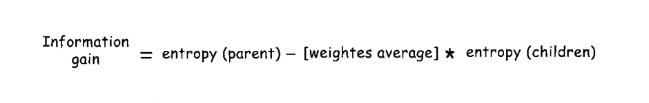
Let’s look at an example to demonstrate how to calculate Information Gain.

Let’s say a set of 30 people both Male and female are split according to their age. Each person’s age is compared to 30 and they are separated into 2 child groups as shown in the image and their corresponding node’s entropy is calculated.

Consider an example where we are building a decision tree to predict whether a loan given to a person would result in a write-off or not. Our entire population consists of 30 instances. 16 belong to the write-off class and the other 14 belong to the non-write-off class. We have two features, namely “Balance” that can take on two values -> “< 50K” or “>50K” and “Residence” that can take on three values -> “OWN”, “RENT” or “OTHER”.

Feature 1: Balance

Reference

Splitting the parent node on attribute balance gives us 2 child nodes.

Let’s calculate the entropy for the parent node. The parent node is the starting point of the decision tree and it contains the entire dataset. It is not typically chosen by the user, but rather the algorithm starts with the entire dataset as the parent node.

Let’s see how much uncertainty the tree can reduce by splitting on Balance.

Splitting on feature , “Balance” leads to an information gain of 0.37 on our target variable. Let’s do the same thing for the feature, “Residence” to see how it compares.

Feature 2: Residence

Splitting the tree on Residence gives us 3 child nodes.

We already know the entropy for the parent node. We simply need to calculate the entropy after the split to compute the information gain from “Residence”

The information gain from feature, Balance is almost 3 times more than the information gain from Residence!

it means that the feature(Balance) with the higher information gain (0.39) is more informative and should be used to split the data at the next internal node.

Steps to build decision tree using information gain:

Consider following dataset

There is a big puzzle for us. How to decide which attribute/feature will give us a smaller tree?

Reference

Code using Sklearn decision tree:

from sklearn.datasets import load_iris
from sklearn import tree
from matplotlib import pyplot as plt
iris = load_iris()

X = iris.data
y = iris.target

#build decision tree
clf = tree.DecisionTreeClassifier(criterion='entropy', max_depth=4,min_samples_leaf=4)
#max_depth represents max level allowed in each tree, min_samples_leaf minumum samples storable in leaf node

#fit the tree to iris dataset
clf.fit(X,y)

#plot decision tree
fig, ax = plt.subplots(figsize=(6, 6)) #figsize value changes the size of plot
tree.plot_tree(clf,ax=ax,feature_names=['sepal length','sepal width','petal length','petal width'])
plt.show()

output:

We finally have our decision tree!

Reference

# make predictions
predictions = clf.predict([[5, 3.5, 1.3, 0.3]])
print(predictions)

output:

[0]

This means that the decision tree has predicted that the input sample belongs to class 0 (Setosa) based on the training data.

References for better understanding:

Python Machine Learning Decision Tree

Final Note: Thanks for reading! I hope you find this article informative.

Don’t forget to read: Decision Trees — Part 3