An Intuitive Explanation of LSTM

10 min readFeb 21, 2022

Recurrent Neural Networks

Recurrent Neural Networks (RNN) differ from feedforward neural networks by the presence of feedback connections where the flow of information occurs between neurons of the same layer or from higher layer neurons to lower layer neurons.

The presence of feedback connections makes RNNs able to perform tasks that require memory. This is because the network keeps information about its previous status. More specifically, the network at the time t transmits to itself the information to be used at the moment t+1 (together with the external input received in t+1). Therefore, the behavior of the network is influenced by the input it receives at a given instant, and by what happened to the network at the previous instant (in turn influenced by the previous instants).

LSTM Architecture

Long Short-Term Memory (LSTM) is a recurrent neural network architecture designed by Sepp Hochreiter and Jürgen Schmidhuber in 1997.

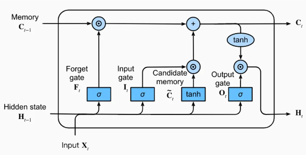
The LSTM architecture consists of one unit, the memory unit (also known as LSTM unit). The LSTM unit is made up of four feedforward neural networks. Each of these neural networks consists of an input layer and an output layer. In each of these neural networks, input neurons are connected to all output neurons. As a result, the LSTM unit has four fully connected layers.

Three of the four feedforward neural networks are responsible for selecting information. They are the forget gate, the input gate, and the output gate. These three gates are used to perform the three typical memory management operations: the deletion of information from memory (the forget gate), the insertion of new information in memory (the input gate), and the use of information present in memory (the output gate).

The fourth neural network, the candidate memory, is used to create new candidate information to be inserted into the memory.

*Figure 1: Architecture of a LSTM Unit (Credits:* https://d2l.ai/chapter_recurrent-modern/lstm.html)

Input and Output

An LSTM unit receives three vectors (three lists of numbers) as input. Two vectors come from the LSTM itself and were generated by the LSTM at the previous instant (instant t − 1). These are the cell state (C) and the hidden state (H). The third vector comes from outside. This is the vector X (called input vector) submitted to the LSTM at instant t.

Given the three input vectors (C, H, X), the LSTM regulates, through the gates, the internal flow of information and transforms the values of the cell state and hidden state vectors. Vectors that will be part of the LSTM input set in the next instant (instant t+ 1). Information flow control is done so that the cell state acts as a long-term memory, while the hidden state acts as a short-term memory.

In practice, the LSTM unit uses recent past information (the short-term memory, H) and new information coming from the outside (the input vector, X) to update the long-term memory (cell state, C). Finally, it uses the long-term memory (the cell state, C) to update the short-term memory (the hidden state, H). The hidden state determined in instant t is also the output of the LSTM unit in instant t. It is what the LSTM provides to the outside for the performance of a specific task. In other words, it is the behavior on which the performance of the LSTM is assessed.

Gates

The three gates (forget gate, input gate and output gate) are information selectors. Their task is to create selector vectors. A selector vector is a vector with values between zero and one and near these two extremes.

A selector vector is created to be multiplied, element by element, by another vector of the same size. This means that a position where the selector vector has a value equal to zero completely eliminates (in the multiplication element by element) the information included in the same position in the other vector. A position where the selector vector has a value equal to one leaves unchanged (in the multiplication element by element) the information included in the same position in the other vector.

All three gates are neural networks that use the sigmoid function as the activation function in the output layer. The sigmoid function is used to have, as output, a vector composed of values between zero and one and near these two extremes.

All three gates use the input vector (X) and the hidden state vector coming from the previous instant (H_[t−1]) concatenated together in a single vector. This vector is the input of all three gates.

Forget Gate

At any time t, an LSTM receives an input vector (X_[t]) as an input. It also receives the hidden state (H_[t−1]) and cell state (C_[t−1]) vectors determined in the previous instant (t− 1).

The first activity of the LSTM unit is executed by the forget gate. The forget gate decides (based on X_[t] and H_[t−1] vectors) what information to remove from the cell state vector coming from time t− 1. The outcome of this decision is a selector vector.

The selector vector is multiplied element by element with the vector of the cell state received as input by the LSTM unit. This means that a position where the selector vector has a value equal to zero completely eliminates (in the multiplication) the information included in the same position in the cell state. A position where the selector vector has a value equal to one leaves unchanged (in the multiplication) the information included in the same position in the cell state.

Input Gate and Candidate Memory

After removing some of the information from the cell state received in input (C_[t−1]), we can insert a new one. This activity is carried out by two neural networks: the candidate memory and the input gate. The two neural networks are independent of each other. Their input are the vectors X_[t] and H_[t−1], concatenated together into a single vector.

The candidate memory is responsible for the generation of a candidate vector: a vector of information that is candidate to be added to the cell state.

Candidate memory output neurons use hyperbolic tangent function. The properties of this function ensure that all values of the candidate vector are between -1 and 1. This is used to normalize the information that will be added to the cell state.

The input gate is responsible for the generation of a selector vector which will be multiplied element by element with the candidate vector.

The selector vector and the candidate vector are multiplied with each other, element by element. This means that a position where the selector vector has a value equal to zero completely eliminates (in the multiplication) the information included in the same position in the candidate vector. A position where the selector vector has a value equal to one leaves unchanged (in the multiplication) the information included in the same position in the candidate vector.

The result of the multiplication between the candidate vector and the selector vector is added to the cell state vector. This adds new information to the cell state.

The cell state, after being updated by the operations we have seen, is used by the output gate and passed into the input set used by the LSTM unit in the next instant (t+ 1).

Output Gate

The output gate determines the value of the hidden state outputted by the LSTM (in instant t) and received by the LSTM in the next instant (t+ 1) input set.

Output generation also works with a multiplication between a selector vector and a candidate vector. In this case, however, the candidate vector is not generated by a neural network, but it is obtained simply by using the hyperbolic tangent function on the cell state vector. This step makes the vector values of the cell state normalized within a range of -1 to 1. In this way, after multiplying with the selector vector (whose values are between zero and one), we get a hidden state with values between -1 and 1. This makes it possible to control the stability of the network over time.

The selector vector is generated from the output gate based on the values of X_[t] and H_[t−1] it receives as input. The output gate uses the sigmoid function as the activation function of the output neurons.

Backpropagation Through Time

The output Y of a neural network depends on a flow of information that passes through many elements placed in a chain. Each of these elements is made in such a way that a small increase in its output value affects the increase (or the decrease) of the output value of all subsequent elements until the output of the network (Y). The error minimization is done by calculating the ratio between the increase in the output value of a particular element and the increase in the network error. This activity is known as Backpropagation.

The backpropagation allows the calculation of the error gradient. For functions with different inputs, the gradient generalizes the concept of derivative. The notion of derivative formalizes the idea of ratio between (instantaneous and infinitely small) increments.

Backpropagation exploits the mathematical technique of the chain rule. The intuition behind the chain rule is: if the error E grows twice as fast as the growth of Y, and Y grows twice as fast as the growth of D, then we can conclude that the error E grows four times as fast as a growth of D. We get to this conclusion by multiplying two ratios (two derivatives).

In RRNs, the flow of information does not occur only through elements of the neural network. It also happens over time. The error committed by the network at the time t also depends on the information received from previous times and processed in these instants of time. In a RRN, therefore, backpropagation also considers the chain of dependencies between instants of time. For this reason, it is called Backpropagation Through Time (BPTT).

RNNs and Long-term Memory

In the basic RRN architecture, the flow of information over time is performed so that the product determined by the application of the chain rule (during backpropagation through time) consists of many factors. Generally, if many factors are close to zero, then the product will be very close to zero. On the other hand, many factors greater than one can result in a very large product.

The study of RNNs highlights how, in the basic RNN architecture, as the time instants considered increase, the product chain determined by backpropagation through time tends to zero or tends to extremely large values. In the first case, we have a vanishing gradient, in the second case an exploding gradient.

Learning occurs by changing the weights of a network in the opposite direction to what is calculated in the product chains of backpropagation through time. This is because, if an increase in a weight causes an increase in the error, then we can reduce the error by decreasing the weight (changing it in the opposite direction of the increase). Therefore, vanishing and exploding gradients have an impact on learning. With a vanishing gradient, the modification of the weights is insignificant (it is very close to zero). With an exploding gradient, the task may be computationally impossible.

The vanishing and exploding gradient problems imply that a basic RRN can exhibit only short-term memory-based behaviors, which therefore does not determine very long product chains during backpropagation through time.

The problem of the exploding gradient can be resolved using the technique of the gradient clipping (https://machinelearningmastery.com/how-to-avoid-exploding-gradients-in-neural-networks-with-gradient-clipping/). The problem of the vanishing gradiend is instead of more difficult resolution.

LSTM and Long-term Memory

The LSTM architecture contrasts the vanishing gradient problem by controlling the flow of information through gates. In an LSTM unit, the flow of information is performed so that the error backpropagation through time depends on the cell state. This implies that the error backpropagation through time uses, as factors (in the product chains), the ratio of (instantaneous and infinitesimal) growths between the cell state in an instant of time and the cell state of the previous instant (∂C_[t]/∂C_[t−1]). The architecture of an LSTM is in such a way that this ratio is the sum of the effects of the four neural networks (the gates and the memory candidate). An LSTM learns (during the learning phase) how to control these effects.

From a mathematical point of view, the previous observation means that an LSTM is able to control the values in the product chains generated by the backpropagation through time: the LSTM can learn how to regulate the effects of the four networks on the ∂C_[t]/∂C_[t−1] factors in order to govern the behavior of the final product (in a product chain generated by backpropagation through time).

The ability to learn to control product chains generated by backpropagation through time allows the LSTM architecture to contrast the vanishing gradient problem. For this reason, the LSTM architecture is able to exhibit not only short-term memory-based behaviors, but also long-term memory-based ones.