The Minimum Mean Absolute Error (MAE) Challenge
Preamble
Several different types of errors can be calculated for regression algorithms, including the mean-squared error (MSE), root mean-squared error (RMSE), and the mean absolute error (MAE)
The errors are the difference between the actual historical data and the forecast-fitted data predicted by the model.

MSE is an absolute error measure that squares the errors (as defined above) to keep the positive and negative errors from canceling each other out. This measure also tends to exaggerate large errors by weighting the large errors more heavily than smaller errors by squaring them, which can help when comparing different time-series models. MSE is calculated by simply taking the average of the Error².

RMSE is the square root of MSE and is the most popular error measure, also known as the quadratic loss function. RMSE can be defined as the average of the absolute values of the forecast errors and is highly appropriate when the cost of the forecast errors is proportional to the absolute size of the forecast error.

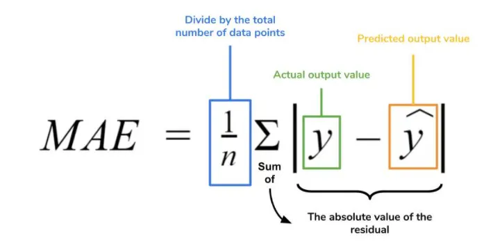
MAE is an error statistic that averages the distance (absolute value of the difference between the actual historical data and the forecast-fitted data predicted by the model) between each pair of actual and fitted forecast data points. MAE is calculated by taking the average of the |Error|, and is most appropriate when the cost of forecast errors is proportional to the absolute size of the forecast errors.

The Goal
With this in mind, I was asked today by some company to solve a classic regression problem.
I am expected to collect relevant data, build a (useful) prediction model, estimate the expected error and off course to explain the CEO what he is paying for.
With this in mind, this is what we are going to do today: Learning how to find the best machine learning model which predicts the company desired target variable (Which is in fact a continuous value and after all we are dealing with a regression problem) with the minimum expected error. Let’s get started!
The Data
The concrete data set was originated from the company and can be downloaded from here.
import pandas as pd
import numpy as np
import matplotlib.pyplot as plt
from sklearn.metrics import mean_absolute_errorconcrete = pd.read_csv("gv_data1.csv")
print(concrete.columns)
Index(['num', 't', 'area_osc', 'Peak.us', 'FT.1', 'FT.3', 'FT.5', 'FT.7', 'FT.9', 'Tag.Mpa', 'sid', 'fname'], dtype='object')
concrete.head()
The concrete data set consists of 798 data points, with 12 features each:
print(“dimension of concrete data: {}”.format(concrete.shape))dimension of concrete data: (798, 12)
“Tag.Mpa” is the feature we are going to predict:
concrete[‘Tag.Mpa’].describe()
The count, mean, min and max rows are self-explanatory. The std shows the standard deviation, and the 25%, 50% and 75% rows show the corresponding percentiles.
import seaborn as snssns.distplot(concrete[‘Tag.Mpa’],kde=True, kde_kws={“color”:”tab:blue”}, hist_kws={“color”:”tab:orange”})

concrete.info()
There are several features that we do not need, such as “num”, “t”, “sid, “fname”, so, we will drop them.
concrete.drop([‘num’,’t’,’sid’,’fname’], axis=1, inplace=True)
concrete.head()
Let’s split the data to X (i.e., features) and y (i.e., target):
X = concrete[ [‘area_osc’,’Peak.us’,’FT.1',’FT.3',’FT.5',’FT.7',’FT.9'] ]
y = concrete[‘Tag.Mpa’]
k-Nearest Neighbors
The k-NN algorithm is arguably the simplest machine learning algorithm. Building the model consists only of storing the training data set. To make a prediction for a new data point, the algorithm finds the closest data points in the training data set — its “nearest neighbors.”
First, Let’s investigate whether we can confirm the connection between model complexity and expected error:
from sklearn.model_selection import train_test_split
X_train, X_test, y_train, y_test = train_test_split(X, y, test_size=0.33, random_state=42)from sklearn.neighbors import KNeighborsRegressortraining_mae = []
test_mae = []# try n_neighbors from 1 to 10
neighbors_settings = range(1, 11)
for n_neighbors in neighbors_settings:
 # build the model
 knn = KNeighborsRegressor(n_neighbors=n_neighbors)
 knn.fit(X_train, y_train)
 y_pred = knn.predict(X_train)
 # record training set expected error
 training_mae.append(mean_absolute_error(y_train, y_pred))
 # record test set expected error
 y_pred1 = knn.predict(X_test)
 test_mae.append(mean_absolute_error(y_test, y_pred1))

plt.plot(neighbors_settings, training_mae, label=”training MAE”)
plt.plot(neighbors_settings, test_mae, label=”test MAE”)
plt.ylabel(“MAE”)
plt.xlabel(“n_neighbors”)
plt.legend()

The above plot shows the training and test set MAE on the y-axis against the setting of n_neighbors on the x-axis. Considering if we choose one single nearest neighbor, the prediction on the training set is perfect. But when more neighbors are considered, the training MAE jumps, indicating that using the single nearest neighbor leads to a model that is too complex. The best performance is somewhere around 6 neighbors.
The plot suggests that we should choose n_neighbors=6. Here we are:
knn = KNeighborsRegressor(n_neighbors=6)
knn.fit(X_train, y_train)y_pred = knn.predict(X_train)
y_pred1 = knn.predict(X_test)
k1 = mean_absolute_error(y_train, y_pred)
k2 = mean_absolute_error(y_test, y_pred1)print(“MAE of KNN Regressor on training set: {:.3f}”.format(k1))
print(“MAE of KNN Regressor on test set: {:.3f}”.format(k2))
MAE of KNN Regressor on training set: 5.821
MAE of KNN Regressor on test set: 7.955
Linear regression
Linear Regression is one of the most common regression algorithms.
from sklearn.linear_model import LinearRegression
linreg = LinearRegression()
linreg.fit(X_train, y_train)y_pred = linreg.predict(X_train)
y_pred1 = linreg.predict(X_test)
l1 = mean_absolute_error(y_train, y_pred)
l2 = mean_absolute_error(y_test, y_pred1)print(“MAE of Linear Regression on training set: {:.3f}”.format(l1))
print(“MAE of Linear Regression on test set: {:.3f}”.format(l2))
MAE of Linear Regression on training set: 6.065
MAE of Linear Regression on test set: 6.576
The linear regression gives us a MAE of 6.06 (in the units of the target variable) on the training and a MAE of 6.58 on the test set.
Decision Tree
A decision tree is a simple, decision making-diagram.
concrete_features = [x for i,x in enumerate(X.columns) if i!=7]from sklearn.tree import DecisionTreeRegressor
tree = DecisionTreeRegressor(random_state=42)
tree.fit(X_train, y_train)y_pred = tree.predict(X_train)
y_pred1 = tree.predict(X_test)
t1 = mean_absolute_error(y_train, y_pred)
t2 = mean_absolute_error(y_test, y_pred1)print(“MAE of Decision Tree Regressor on training set: {:.3f}”.format(t1))
print(“MAE of Decision Tree Regressor on test set: {:.3f}”.format(t2))
MAE of Decision Tree Regressor on training set: 0.000
MAE of Decision Tree Regressor on test set: 4.208
The MAE on the training set is 0.000, while the test set MAE is much worse. This is an indicative that the tree is overfitting and not generalizing well to new data. Therefore, we need to apply pre-pruning to the tree.
We set max_depth=11, limiting the depth of the tree decreases overfitting. This leads to a higher MAE on the training set, but an improvement on the test set.
tree1 = DecisionTreeRegressor(random_state=42, max_depth=11)
tree1.fit(X_train, y_train)y_pred = tree1.predict(X_train)
y_pred1 = tree1.predict(X_test)
t3 = mean_absolute_error(y_train, y_pred)
t4 = mean_absolute_error(y_test, y_pred1)print(“MAE of Decision Tree Regressor on training set: {:.3f}”.format(t3))
print(“MAE of Decision Tree Regressor on test set: {:.3f}”.format(t4))
MAE of Decision Tree Regressor on training set: 0.593
MAE of Decision Tree Regressor on test set: 4.190
Feature Importance in Decision Trees
Feature importance rates how important each feature is for the decision a tree makes. It is a number between 0 and 1 for each feature, where 0 means “not used at all” and 1 means “perfectly predicts the target”. The feature importances always sum to 1:
print(“Feature importances:\n{}”.format(tree1.feature_importances_))Feature importances: [0.0798353 0.28033977 0.06243741 0.03522198 0.03051368 0.05825283 0.45339904]
Then we can visualize the feature importances:
def plot_feature_importances(model):
 plt.figure(figsize=(8,6))
 n_features = X.shape[1]
 plt.barh(range(n_features), model.feature_importances_, align=’center’)
 plt.yticks(np.arange(n_features), concrete_features)
 plt.xlabel(“Feature importance”)
 plt.ylabel(“Feature”)
 plt.ylim(-1, n_features)plot_feature_importances(tree1)
plt.savefig(‘feature_importance’)

Feature “FT.9” is by far the most important feature.
Random Forest
Random forests are a large number of trees, combined (using averages or “majority rules”) at the end of the process. Let’s apply a random forest consisting of 100 trees on the concrete data set:
from sklearn.ensemble import RandomForestRegressor
rf = RandomForestRegressor(random_state=42, n_estimators=100)
rf.fit(X_train, y_train)y_pred = rf.predict(X_train)
y_pred1 = rf.predict(X_test)
r1 = mean_absolute_error(y_train, y_pred)
r2 = mean_absolute_error(y_test, y_pred1)print(“MAE of Random Forest Regressor on training set: {:.3f}”.format(r1))
print(“MAE of Random Forest Regressor on test set: {:.3f}”.format(r2))
MAE of Random Forest Regressor on training set: 1.428
MAE of Random Forest Regressor on test set: 3.351
The random forest gives us an MAE of 3.351, better than the linear regression model or a single decision tree, without tuning any parameters. However, we can adjust the max_features setting, to see whether the result can be improved.
rf1 = RandomForestRegressor(random_state=42, n_estimators=100, max_depth=11)
rf1.fit(X_train, y_train)y_pred = rf1.predict(X_train)
y_pred1 = rf1.predict(X_test)
r3 = mean_absolute_error(y_train, y_pred)
r4= mean_absolute_error(y_test, y_pred1)print(“MAE of Random Forest Regressor on training set: {:.3f}”.format(r3))
print(“MAE of Random Forest Regressor on test set: {:.3f}”.format(r4))
MAE of Random Forest Regressor on training set: 1.529
MAE of Random Forest Regressor on test set: 3.395
It did not, this indicates that the default parameters of the random forest work well.
Feature importance in Random Forest
plot_feature_importances(rf)
Similarly, to the single decision tree, the random forest also gives a lot of importance to the “FT.9” feature, and also chooses “Peak.us” to be the 2nd most informative feature overall. The randomness in building the random forest forces the algorithm to consider many possible explanations, the result being that the random forest captures a much broader picture of the data than a single tree.
Gradient Boosting
Gradient boosting machines also combine decision trees, but start the combining process at the beginning, instead of at the end.
from sklearn.ensemble import GradientBoostingRegressor
gb = GradientBoostingRegressor(random_state=42)
gb.fit(X_train, y_train)y_pred = gb.predict(X_train)
y_pred1 = gb.predict(X_test)
g1 = mean_absolute_error(y_train, y_pred)
g2 = mean_absolute_error(y_test, y_pred1)print(“MAE of Gradient Boosting Regressor on training set: {:.3f}”.format(g1))
print(“MAE of Gradient Boosting Regressor on test set: {:.3f}”.format(g2))
MAE of Gradient Boosting Regressor on training set: 2.355
MAE of Gradient Boosting Regressor on test set: 3.634
We are likely to be overfitting. To reduce overfitting, we could either apply stronger pre-pruning by limiting the maximum depth or lower the learning rate:
gb1 = GradientBoostingRegressor(random_state=42, max_depth=1)
gb1.fit(X_train, y_train)y_pred = gb1.predict(X_train)
y_pred1 = gb1.predict(X_test)
g3 = mean_absolute_error(y_train, y_pred)
g4 = mean_absolute_error(y_test, y_pred1)print(“MAE of Gradient Boosting Regressor on training set: {:.3f}”.format(g3))
print(“MAE of Gradient Boosting Regressor on test set: {:.3f}”.format(g4))
MAE of Gradient Boosting Regressor on training set: 4.373
MAE of Gradient Boosting Regressor on test set: 4.781
gb2 = GradientBoostingRegressor(random_state=42, learning_rate=0.01)
gb2.fit(X_train, y_train)y_pred = gb2.predict(X_train)
y_pred1 = gb2.predict(X_test)
g5 = mean_absolute_error(y_train, y_pred)
g6 = mean_absolute_error(y_test, y_pred1)print(“MAE of Gradient Boosting Regressor on training set: {:.3f}”.format(g5))
print(“MAE of Gradient Boosting Regressor on test set: {:.3f}”.format(g6))
MAE of Gradient Boosting Regressor on training set: 5.482
MAE of Gradient Boosting Regressor on test set: 6.072
Both methods of decreasing the model complexity increased the training set MAE, as expected. However, in this case, none of these methods decreased the MAE of the test set.
We can visualize the feature importances of the first model (“out of the box”):
plot_feature_importances(gb)
We can see that the feature importances of the gradient boosted trees are similar to the feature importances of the random forests.
Support Vector Machine
Linear Regression has explicit decision and SVM finds approximate of real decision because of numerical (computational) solution. While linear regression models minimize the error between the actual and predicted values through the line of best fit, SVM manages to fit the best line within a threshold of values, otherwise called the epsilon-insensitive tube.
from sklearn.svm import SVR
svr = SVR()
svr.fit(X_train, y_train)y_pred = svr.predict(X_train)
y_pred1 = svr.predict(X_test)
s1 = mean_absolute_error(y_train, y_pred)
s2 = mean_absolute_error(y_test, y_pred1)print(“MAE of Support Vector Regressor on training set: {:.3f}”.format(s1))
print(“MAE of Support Vector Regressor on test set: {:.3f}”.format(s2))
MAE of Support Vector Regressor on training set: 7.704
MAE of Support Vector Regressor on test set: 8.707
SVM requires all the features to vary on a similar scale, and ideally to have a minimum value of 0, and a maximum value of 1. We will need to re-scale our data that all the features are approximately on the same scale:
from sklearn.preprocessing import MinMaxScalerscaler = MinMaxScaler()
X_train_scaled = scaler.fit_transform(X_train)
X_test_scaled = scaler.fit_transform(X_test)svr1 = SVR()
svr1.fit(X_train_scaled, y_train)y_pred = svr1.predict(X_train_scaled)
y_pred1 = svr1.predict(X_test_scaled)
s3 = mean_absolute_error(y_train, y_pred)
s4 = mean_absolute_error(y_test, y_pred1)print(“MAE of Support Vector Regressor on training set: {:.3f}”.format(s3))
print(“MAE of Support Vector Regressor on test set: {:.3f}”.format(s4))
MAE of Support Vector Regressor on training set: 5.355
MAE of Support Vector Regressor on test set: 6.390
Scaling the data made a huge difference! From here, we can try increasing either C or gamma to fit a more complex model.
svr2 = SVR(gamma=10)
svr2.fit(X_train_scaled, y_train)y_pred = svr2.predict(X_train_scaled)
y_pred1 = svr2.predict(X_test_scaled)
s5 = mean_absolute_error(y_train, y_pred)
s6 = mean_absolute_error(y_test, y_pred1)print(“MAE of Support Vector Regressor on training set: {:.3f}”.format(s5))
print(“MAE of Support Vector Regressor on test set: {:.3f}”.format(s6))
MAE of Support Vector Regressor on training set: 5.021
MAE of Support Vector Regressor on test set: 5.872
Here, increasing C allows us to improve the model, resulting in a MAE of 5.872 on the test set.
Deep Learning
A multilayer perceptron (MLP) is a feedforward artificial neural network that generates a set of outputs from a set of inputs. An MLP is characterized by several layers of input nodes connected as a directed graph between the input and output layers. MLP uses backpropagation for training the network.
from sklearn.neural_network import MLPRegressor
mlp = MLPRegressor(random_state=42)
mlp.fit(X_train, y_train)y_pred = mlp.predict(X_train)
y_pred1 = mlp.predict(X_test)
m1 = mean_absolute_error(y_train, y_pred)
m2 = mean_absolute_error(y_test, y_pred1)print(“MAE of MLP Regressor on training set: {:.3f}”.format(m1))
print(“MAE of MLP Regressor on test set: {:.3f}”.format(m2))
MAE of MLP Regressor on training set: 8.439
MAE of MLP Regressor on test set: 9.663
The MAE of the Multilayer perceptrons (MLP) is higher than those of the other models, this is likely due to scaling of the data. deep learning algorithms also expect all input features to vary in a similar way, and ideally to have a mean of 0, and a variance of 1. We must re-scale our data so that it fulfills these requirements.
from sklearn.preprocessing import StandardScaler
scaler = StandardScaler()
X_train_scaled = scaler.fit_transform(X_train)
X_test_scaled = scaler.fit_transform(X_test)mlp1 = MLPRegressor(random_state=42)
mlp1.fit(X_train_scaled, y_train)y_pred = mlp1.predict(X_train_scaled)
y_pred1 = mlp1.predict(X_test_scaled)
m3 = mean_absolute_error(y_train, y_pred)
m4 = mean_absolute_error(y_test, y_pred1)
print(“MAE of MLP Regressor on training set: {:.3f}”.format(m3))
print(“MAE of MLP Regressor on test set: {:.3f}”.format(m4))
MAE of MLP Regressor on training set: 6.635
MAE of MLP Regressor on test set: 7.018
Let’s increase the number of iterations:
mlp2 = MLPRegressor(random_state=42, max_iter=1000)
mlp2.fit(X_train_scaled, y_train)y_pred = mlp2.predict(X_train_scaled)
y_pred1 = mlp2.predict(X_test_scaled)
m5 = mean_absolute_error(y_train, y_pred)
m6 = mean_absolute_error(y_test, y_pred1)print(“MAE of MLP Regressor on training set: {:.3f}”.format(m5))
print(“MAE of MLP Regressor on test set: {:.3f}”.format(m6))
MAE of MLP Regressor on training set: 4.069
MAE of MLP Regressor on test set: 4.510
Increasing the number of iterations decreased both the training set MAE and the test set MAE.
mlp3 = MLPRegressor(random_state=42, max_iter=1000, alpha=1)
mlp3.fit(X_train_scaled, y_train)y_pred = mlp3.predict(X_train_scaled)
y_pred1 = mlp3.predict(X_test_scaled)
m7 = mean_absolute_error(y_train, y_pred)
m8 = mean_absolute_error(y_test, y_pred1)print(“MAE of MLP Regressor on training set: {:.3f}”.format(m7))
print(“MAE of MLP Regressor on test set: {:.3f}”.format(m8))
MAE of MLP Regressor on training set: 4.075
MAE of MLP Regressor on test set: 4.547
The result is good, but we are not able to decrease the test MAE further.
Therefore, our best model so far is the deep learning model after scaling and with 1,000 iterations.
Finally, we plot a heat map of the first layer weights in a neural network learned on the concrete data set.
plt.figure(figsize=(20, 5))
plt.imshow(mlp2.coefs_[0], interpolation=’none’, cmap=’viridis’)
plt.yticks(range(X.shape[1]), concrete_features)
plt.xlabel(“Columns in weight matrix”)
plt.ylabel(“Input feature”)
plt.colorbar()
From the heat map, it is not easy to point out quickly that which feature (features) have relatively low weights compared to the other features.
Conclusion
models = [“KNN Regressor”, “Linear Regression”, “Decision Tree Regressor” ,”Random Forest Regressor”, “Gradient Boosting Regressor”,”Support Vector Regressor”, “MLP Regressor”]
tests_mae = [k2, l2, t4, r2, g2, s6, m6]
compare_models = pd.DataFrame({ “Algorithms”: models, “Tests MAE”: tests_mae })
compare_models.sort_values(by = “Tests MAE”, ascending = True)
Of all the models we trained and tested, the model with the lowest expected error (in absolute values and in terms of the target variable) was the random tree with an expected error of 3.351.
import matplotlib.pyplot as plt
%matplotlib inline
plt.figure(figsize=(8,8))
sns.barplot(x = “Tests MAE”, y = “Algorithms”, data = compare_models)
plt.show()
Done! We now have a working Random Forest prediction model.
The Chosen Model
Let’s calculate the R squared of the chosen model:
from sklearn.metrics import r2_scorerf = RandomForestRegressor(random_state=42, n_estimators=100)
rf.fit(X_train, y_train)y_pred = rf.predict(X_test)
print("Random Forest R squared: {:.4f}".format(r2_score(y_test, y_pred)))
Random Forest R squared: 0.8639
So, in our model, 86.39% of the variability in Y can be explained using X. This is very exciting.
Let‘s inspect the differences in a DataFrame. First, we concatenate the true and predicted Tag.Mpa:
y_test1 = y_test.copy()
gross = []
for i in y_pred:
 gross.append(i)
df = pd.DataFrame(data=gross)
df = df.set_index(y_test1.index)
df.rename(columns={0: “predicted”}, inplace=True)
df1 = pd.concat([y_test1, df ], axis=1)
df1.columns = [“true”, “predicted”]
df1.head()
And compute the difference score, which will show us if more values are positive or negative:
df1[“diff”] = df1[“predicted”] — df1[“true”]
df1.head()
There is a tendency for the Tag.Mpa test values being underestimated, as we can see in the histogram:
plt.hist(df1[“diff”], bins=26, color=”pink”, edgecolor=”brown”, linewidth=1.2)
plt.axvline(0, color=”red”, linestyle=”dashed”, linewidth=1.6)
plt.show()
And the below table confirms this as well:
pd.DataFrame({“Count”: [(df1[“diff”]<0).sum(), (df1[“diff”]==0).sum(),(df1[“diff”]>0).sum()]}, columns=[“Count”],index=[“Underestimation”, “Exact Estimation”, “Overestimation”])
In many data science projects, slight underestimation is not a real problem.
Let’s calculate the mean square error (MSE) of the chosen model:
df1[“Squared Error”] = 0.00
df1[“Squared Error”] = ( df1[‘true’] — df1[‘predicted’] )**2
MSE = np.mean(df1[“Squared Error”])
print(“Random Forest MSE: {:.4f}”.format(MSE))
Random Forest MSE: 20.0613
This number as no physical meaning only mathematical one.
Let’s calculate the root-mean square error (RMSE) of the chosen model:
RMSE = np.sqrt(np.mean(df1["Squared Error"]))
print("Random Forest RMSE: {:.4f}".format(RMSE))
Random Forest RMSE: 4.4790
Our model was able to predict the Tag.Mpa of every record in the test set within ±4.4790 of the real Tag.Mpa value (using Euclidean distances).
Let’s calculate the mean absolute error (MAE) of the chosen model, which is our metric for the expected error in absolute terms:
df1["Absolute Error"] = 0.00
df1["Absolute Error"] = abs( df1['true'] - df1['predicted'] )
MAE = np.mean(df1["Absolute Error"])
print("Random Forest MAE: {:.4f}".format(MAE))
Random Forest MAE: 3.3511
Our model was able to predict the Tag.Mpa of every record in the test set within ±3.3511 of the real Tag.Mpa value (using Manhattan distances).
Finally, let’s calculate the mean squared logarithmic error (MSLE) of the chosen model, which is our metric for the expected error in percentage terms:
from sklearn.metrics import mean_squared_log_errorMSLE = mean_squared_log_error(y_test, y_pred)print("Random Forest MSLE: {:.4%}".format(MSLE))
Random Forest MSLE: 2.3770%
Our model was able to predict the Tag.Mpa of every record in the test set within ±2.3770% from the real Tag.Mpa value (using Euclidean distances).
Summary
We practiced a wide array of machine learning models for regression, what their advantages and disadvantages are, and how to control model complexity for each of them. We saw that for many of the algorithms, setting the right parameters is important for minimum expected error.
We should be able to know how to apply, tune, and analyze the models we practiced above. It’s your turn now! Try applying any of these algorithms to the built-in data sets in scikit-learn or any data set at your choice. Happy Machine Learning!
Source code that created this post can be found here. I would be pleased to receive feedback or questions on any of the above.
About the Author

Roi Polanitzer, PDS, ADL, MLS, PDA, CPD, F.IL.A.V.F.A., FRM, is a data scientist with an extensive experience in solving machine learning problems, such as: regression, classification, clustering, recommender systems, anomaly detection, text analytics & NLP, and image processing. Mr. Polanitzer is is the Owner and Chief Data Scientist of Prediction Consultants — Advanced Analysis and Model Development, a data science firm headquartered in Rishon LeZion, Israel. He is also the Owner and Chief Appraiser of Intrinsic Value — Independent Business Appraisers, a business valuation firm that specializes in corporates, intangible assets and complex financial instruments valuation.
Over more than 16 years, he has performed data science projects such as: regression (e.g., house prices, CLV- customer lifetime value, and time-to-failure), classification (e.g., market targeting, customer churn), probability (e.g., spam filters, employee churn, fraud detection, loan default, and disease diagnostics), clustering (e.g., customer segmentation, and topic modeling), dimensionality reduction (e.g., p-values, itertools Combinations, principal components analysis, and autoencoders), recommender systems (e.g., products for a customer, and advertisements for a surfer), anomaly detection (e.g., supermarkets’ revenue and profits), text analytics (e.g., identifying market trends, web searches), NLP (e.g., sentiment analysis, cosine similarity, and text classification), image processing (e.g., image binary classification of dogs vs. cats, , and image multiclass classification of digits in sign language), and signal processing (e.g., audio binary classification of males vs. females, and audio multiclass classification of urban sounds).
Mr. Polanitzer holds various professional designations, such as a global designation called “Financial Risk Manager” (FRM, which indicates that its holder is proficient in developing, implementing and validating statistical models and mathematical algorithms such as K-Means, SVM and KNN for credit risk measurement and management) from the Global Association of Risk Professionals (GARP), a designation called “Fellow Actuary” (F.IL.A.V.F.A., which indicates that its holder is proficient in developing, implementing and validating statistical models and mathematical algorithms such as GLM, RF and NN for determining premiums in general insurance) from the Israel Association of Valuators and Financial Actuaries (IAVFA), and a designation called “Certified Risk Manager” (CRM, which indicates that its holder is proficient in developing, implementing and validating statistical models and mathematical algorithms such as DT, NB and PCA for operational risk management) from the Israeli Association of Risk Managers (IARM).
Mr. Polanitzer had studied actuarial science (i.e., implementation of statistical and data mining techniques for solving time-series analysis, dimensionality reduction, optimization and simulation problems) at the prestigious 250-hours training program of the University of Haifa, financial risk management (i.e., building statistical predictive and probabilistic models for solving regression, classification, clustering and anomaly detection) at the prestigious 250-hours training program of the program of the Ariel University, and machine learning and deep learning (i.e., building recommender systems and training neural networks for image processing and NLP) at the prestigious 500-hours training program of the John Bryce College.
He had graduated various professional trainings at the John Bryce College, such as: “Introduction to Machine Learning, AI & Data Visualization for Managers and Architects”, “Professional training in Practical Machine Learning, AI & Deep Learning with Python for Algorithm Developers & Data Scientists”, “Azure Data Fundamentals: Relational Data, Non-Relational Data and Modern Data Warehouse Analytics in Azure”, and “Azure AI Fundamentals: Azure Tools for ML, Automated ML & Visual Tools for ML and Deep Learning”.
Mr. Polanitzer had also graduated various professional trainings at the Professional Data Scientists’ Israel Association, such as: “Neural Networks and Deep Learning”, “Big Data and Cloud Services”, “Natural Language Processing and Text Mining”.