UNDERSTANDING CRYPTO ECONOMIC CYCLES USING BLOCKCHAIN DATA FROM SANTIMENT
Introduction
It is standard practice in conventional economic studies to collect multi-year data and then analyse it to understand the economic cycles using multiple approaches for investment and trading strategies. But the data for conventional economic systems is always compromised. Therefore, the integrity and quality of data affects the outcomes of these studies.
Crypto economy is very new and evolving. With time the dataset that is available for crypto assets is much richer in attributes than what is available for conventional economy. More important is — all the data is always available on the blockchain and is never compromised. Therefore, the results of the studies from such data will be free of issues due to quality and integrity of the data.
Santiment, a Switzerland based company with its smart contract on the Ethereum blockchain, was launched in H1'2017. The Santiment team has developed a large number of features for each crypto asset, particularly ERC20 assets, and can be accessed by anybody from their platform.
ShilazTech, an India based company, specializes in analysing large data sets using machine learning to identify patterns for developing investment and trading strategies.
Santiment and ShilazTech joined hands to study the available data for the leading blockchains, Bitcoin and Ethereum, with the objective to understand the relatively long period crypto economic cycles and use that understanding to build investment and trading strategies. A parallel objective is to let crypto enthusiasts know about the wealth of information available on blockchains that is there and yet to be extracted from the data provided by Santiment.
The date range for the analysis was since its beginning till 5 May 2019 when the study commenced. The final date ranges were adjusted based on the availability of the features. The study is divided into four parts — Review of past studies, Analysis for Bitcoin, Analysis for Ethereum, and Conclusions & Recommendations.
Review of Past Studies
There are many studies that bitcoin researchers have done to understand — what drives bitcoin valuation and price cyclicity. Some of my favourite studies are discussed below in brief:
Hodl Waves
Unchained Capital defines hodl waves as below:
Hodl waves reflect the behaviour of asset hodlers. If a hodler keep holding the asset then it effectively reduces the supply of asset and helps increase the price of the asset. In the case of bitcoin it is possible to compute the time a bitcoin is not moved from an address.
A HODL wave is created when a large amount of Bitcoin transacts on the way up to and through a local price high, becoming recent BTC (1 day — 1 week old), and then slowly ages into each later band as its new owners HODL.
A HODL wave manifests visually on the chart as a pattern of nested curves caused by each age band becoming suddenly much fatter (taller) at progressively later times from the rally.
The image below traces a few of the largest HODL waves.
Unchained Capital in their article Bitcoin Data Science (Pt. 1): HODL Waves has discussed about how the holders behaviour, measured through HODL waves, helps understand valuation and price cyclicity of the bitcoin.
However, the article does not present a decisive methodology for exit and entry from the market based on HODL waves.
Stock Flow Model
PlanB has popularized the stock flow model for bitcoin through his article Modeling Bitcoin’s Value with Scarcity. In this article he quantifies scarcity using stock-to-flow, and uses stock-to-flow to model bitcoin’s value. The confidence in the model increases as Gold and silver, which are totally different markets, are in line with the bitcoin model values for SF.
The model is very good to know when the bitcoin is undervalued or overvalued. Entry points are reasonably picked up by the methodology but fails to provide satisfactory exit points.
Dormancy Model
Adaptive Capital has discussed their dormancy model for bitcoin in the article Bitcoin Average Dormancy. Dormancy is defined as the average number of days destroyed per coin transacted in any given day. In this article they show that Dormancy flow is ideal for both bottom-catching historical global lows and assessing whether the bull market remains in relatively normal conditions as seen in the below figure:
Again this methodology is very good to pick up the bottom but fails to provide decisive exit point.
Mayer Multiple Model
The Mayer Multiple was created by Trace Mayer as a way to analyse the price of Bitcoin in a historical context. The Mayer Multiple is a multiple of the current Bitcoin price over the 200-days moving average. Simulations performed by Trace Mayer determined that in the past, the best long-term results were achieved by accumulating Bitcoin whenever the Mayer Multiple was below 2.4 as shown in the below figure:
This model fails to pinpoint the entry point and has no specific criteria for exit.
Log-Log Model
Harold Christopher Burger in his article Bitcoin’s natural long-term power-law corridor of growth has proposed a log-log model to guestimate the BTC price as a function of time only as shown in the below figure:
In his model he did regression analysis between log of BTC price and log of days since BTC was launched. And he found remarkably linear relation between the two. Linear regression gives power-law to predict the price of bitcoin on a given day.
This model seems to pick up entry as well as exit points. To obtain buy/accumulation zone he has to shift main regression line downward by some adhoc value to define green (accumulation zone) and support line. And to define resistance line or exit points he has to run a separate regression on three ATH points of each bull/bear phase.
MVRV Model
Santiment has developed MVRV model. MVRV is the ratio of market value to realized value. MVRV long/short diff measures the difference between long and short period MVRV. The figure below shows this feature for Bitcoin:
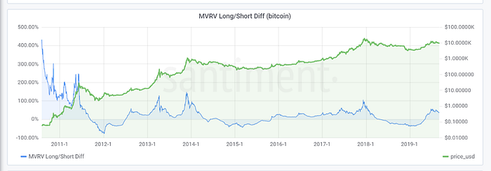
This model also gives reasonably good entry points after each bear phase when MVRV long/short diff crosses above zero. But fails to give exit points.
In conclusion — most studies that have been done, help understand when the bitcoin is undervalued and provides a good entry point. But almost all of them fail to provide satisfactory exit point.
The focus of our study is to be able to get reasonable exit points for large bear/bull cycles in addition to entry points and if possible then pick intercycle entry/exit too.
Analysis for Bitcoin
Bitcoin is now in existence for more than 10 years. The blockdata history of bitcoin since its launch on 3 Jan 2009 are available for anyone to study and analyse. The figure below shows price history for Bitcoin from 17 July 2010 to 5 May 2019.
The price history clearly shows roller coaster behaviour. Although there are large ups and downs, overall there is huge price appreciation since its launch. Therefore, it is of immense value and interest to crypto world to understand the price behaviour and predict the future price levels or changes in price.
We worked on five different approaches:
- Approach 1- predict the value of current daily close price to identify times of under or overvalued zones using backpropagation neural network and utilize that to come up with a simple investment/trading strategy
- Approach 2- predict the value of current close to identify times of under or overvalued zones using LSTM neural network and utilize that to come up with a simple investment/trading strategy
- Approach 3- Use HODL Waves to come up with a simple investment/trading strategy
- Approach 4- predict the percent change of the future n days and utilize that to come up with a simple investment/trading strategy
- Approach 5- Hybrid strategy of above two
We used the following procedure to evaluate the value addition of these approaches:
- Design two trading signals using a simple strategy based on Simple Moving Average (SMA)
- MA Signal with SMA2 (2 Sample) and SMA11 (11 Sample) for actual close
- Filtered Signal by combining
- MA Signal with SMA2 (2 Sample) and SMA11 (11 Sample) for actual close
- MA Signal with SMA2 (2 Sample) and SMA11 (11 Sample) field derived using predicted value
- Take the trade only if both above signal have same signal
- Trading Strategy
- Start Equity 100K
- Brokerage 0.075%
- Today’s Signal to be executed on next day ‘open price’
- Compare the equity gain of filtered signal with MA Signal
- Compare the equity gain of filtered signal with Buy and Hold
- Compare risk return parameters for above two signals
Data Collection
We have used data from two sources — Blockchain.info and Santiment. The date range for the data used is from 28 Apr 2013 to 8 May 2019. Below is the list of data from each source
Data from Blockchain.info
Data from Santiment
AvgBlockSize, Ntransactions, Difficulty, BlocksSize, CostPerTransaction, HashRate, MarketCap, MedianConfirmationTime, NTransactionsperBlock, transactionfees, nuniqueaddresses, estimatedtransactionvolumeusd, MinersRevenue, openPriceUsd, closePriceUsd, highPriceUsd, lowPriceUsd, volume, marketcap, daily_active_addresses, network_growth, burn_rate, token_age_consumed, average_token_age_consumed_in_days, transaction_volume, token_velocity, token_circulation, mvrv_ratio, nvt_ratio, daily_active_deposits, github_activity, dev_activity, exchange_funds_flow, social_volume_PROFESSIONAL_TRADERS_CHAT_OVERVIEW, social_volume_TELEGRAM_CHATS_OVERVIEW, social_volume_DISCORD_DISCUSSION_OVERVIEW, BTC_hodl_waves.csv_circulation_7d, BTC_hodl_waves.csv_circulation_10y, BTC_hodl_waves.csv_circulation_180d, BTC_hodl_waves.csv_circulation_1d, BTC_hodl_waves.csv_circulation_20y, BTC_hodl_waves.csv_circulation_2y, BTC_hodl_waves.csv_circulation_30d, BTC_hodl_waves.csv_circulation_365d, BTC_hodl_waves.csv_circulation_3y, BTC_hodl_waves.csv_circulation_5y, BTC_hodl_waves.csv_circulation_60d, BTC_bounded_mvrv.csv_mvrv_10y, BTC_bounded_mvrv.csv_mvrv_180d, BTC_bounded_mvrv.csv_mvrv_1d, BTC_bounded_mvrv.csv_mvrv_20y, BTC_bounded_mvrv.csv_mvrv_2y, BTC_bounded_mvrv.csv_mvrv_30d, BTC_bounded_mvrv.csv_mvrv_365d, BTC_bounded_mvrv.csv_mvrv_3y, BTC_bounded_mvrv.csv_mvrv_5y, BTC_bounded_mvrv.csv_mvrv_60d, BTC_realized_value.csv_realized_value, BTC_marketcaps.csv_circulation_10y, BTC_marketcaps.csv_circulation_180d, BTC_marketcaps.csv_circulation_1d, BTC_marketcaps.csv_circulation_20y, BTC_marketcaps.csv_circulation_2y, BTC_marketcaps.csv_circulation_30d, BTC_marketcaps.csv_circulation_365d, BTC_marketcaps.csv_circulation_3y, BTC_marketcaps.csv_circulation_5y, BTC_marketcaps.csv_circulation_60d, BTC_active_coins.csv_% of coins active last 3 years, BTC_active_coins.csv_% of coins active last 1 years, BTC_realized_cap.csv_realized_cap_10y , BTC_realized_cap.csv_realized_cap_180d, BTC_realized_cap.csv_realized_cap_1d, BTC_realized_cap.csv_realized_cap_20y, BTC_realized_cap.csv_realized_cap_2y, BTC_realized_cap.csv_realized_cap_30d, BTC_realized_cap.csv_realized_cap_365d, BTC_realized_cap.csv_realized_cap_3y, BTC_realized_cap.csv_realized_cap_5y, BTC_realized_cap.csv_realized_cap_60d, BTC_mvrv_diff.csv_MVRV Long/Short Diff
Both these data sets were merged to make one dataset. And that data set is then utilized for the analysis.
Remove Redundant Features
There are a total of 76 features in the merged file. It is obvious to expect that many of the fields would be highly correlated to each other. Therefore, we did a correlation analysis to find highly correlated fields and remove all those that have correlation greater than 0.95. That gave us those fields that are not correlated to each other. Below is the list of those 33 features:
[‘openPriceUsd’ ‘volume’ ‘daily_active_addresses’ ‘burn_rate’
‘transaction_volume’ ‘token_circulation’ ‘mvrv_ratio’ ‘github_activity’
‘dev_activity’ ‘BTC_hodl_waves.csv_circulation_10y’
‘BTC_hodl_waves.csv_circulation_180d’ ‘BTC_hodl_waves.csv_circulation_2y’
‘BTC_hodl_waves.csv_circulation_30d’
‘BTC_hodl_waves.csv_circulation_365d’ ‘BTC_hodl_waves.csv_circulation_3y’
‘BTC_hodl_waves.csv_circulation_60d’ ‘BTC_bounded_mvrv.csv_mvrv_180d’
‘BTC_bounded_mvrv.csv_mvrv_1d’ ‘BTC_bounded_mvrv.csv_mvrv_30d’
‘BTC_bounded_mvrv.csv_mvrv_60d’ ‘BTC_realized_value.csv_realized_value’
‘BTC_marketcaps.csv_circulation_1d’
‘BTC_active_coins.csv_% of coins active last 3 years’
‘BTC_active_coins.csv_% of coins active last 1 years’
‘BTC_realized_cap.csv_realized_cap_180d’
‘BTC_mvrv_diff.csv_MVRV Long/Short Diff’ ‘AvgBlockSize’ ‘Ntransactions’
‘Difficulty’ ‘BlocksSize’ ‘CostPerTransaction’ ‘MedianConfirmationTime’
‘transactionfees’]
Approach-1
In this approach we try to predict the close price while using other features as input to backpropagation neural network.
In this approach, first we carry out correlation analysis with close to identify and remove those features that are less correlated with close (correlation<0.1). The figure below shows the correlation of selected features with close:

Below is the final list of selected features
Close, volume, daily_active_addresses, mvrv_ratio, github_activity, dev_activity, social_volume_PROFESSIONAL_TRADERS_CHAT_OVERVIEW, social_volume_TELEGRAM_CHATS_OVERVIEW, social_volume_DISCORD_DISCUSSION_OVERVIEW, BTC_hodl_waves_circulation_10y, BTC_hodl_waves_circulation_180d, BTC_hodl_waves_circulation_2y, BTC_hodl_waves_circulation_30d, BTC_hodl_waves_circulation_365d, BTC_hodl_waves_circulation_3y, BTC_hodl_waves_circulation_60d, BTC_active_coins_% of coins active last 3 years, BTC_active_coins_% of coins active last 1 years, AvgBlockSize, Ntransactions, Difficulty, BlocksSize, MedianConfirmationTime
These features are used as input and the close price as output to a backpropagation neural network, with one hidden layer, and the network is trained on data set between 28 Apr 2013 to 8 May 2019. The trained network is then used to model the close. The figure below shows comparison of modelled close with actual close:
The figure below shows the accuracy for modelling the close.
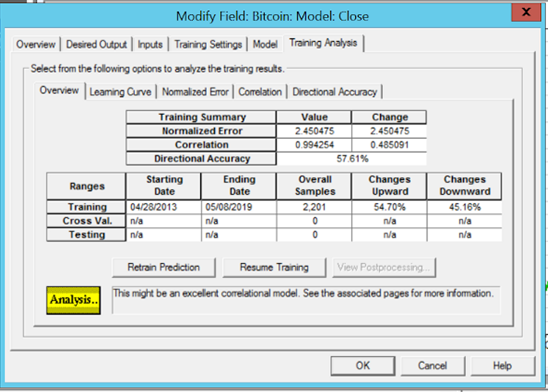
Below are the observations and conclusions from this:
- Modelled close is highly correlated with close (correlation =0.99) while inputs did not have any imprint of close
- Direction accuracy >50% (57%)
- Results are encouraging for further analysis
Walk Forward Simulation
The above modelled close is not suitable to build a trading/investment strategy as in this case entire data was used to train and model the close in one go. So, to simulate the real world scenario we will have to do this modelling in walk forward basis. The close that is modelled through walk forward simulation can be the representative close that can be then used to build a trading strategy.
Below is the procedure for walk forward simulation that we have used:
- Read all the features from merged CSV file
- For walk forward do following
- First simulation
- Select first 365 samples
- Remove all the features that are highly correlated to each other >max correlation threshold (0.95)
- From remaining features remove all the features that are less correlated with close <min correlation threshold (0.1)
- Normalize remaining features as well as output field
- Optimally select neurons in hidden layer, training epochs, and batch size based on number of available samples
- Train the backpropagation neural network
- Predict close for last sample using trained neural network and denormalize output
- Keep the predicted close and merge with previous 364 samples. Call this predicted close
- Second simulation
- Select first 366 samples
- Remove all the features that are highly correlated to each other >max correlation threshold (0.95)
- From remaining features remove all the features that are less correlated with close <min correlation threshold (0.1)
- Normalize remaining features as well as output field
- Optimally select neurons in hidden layer, training epochs, and batch size based on number of available samples
- Train the backpropagation neural network
- Predict close for last sample using trained neural network and denormalize output
- Keep the predicted close and merge with predicted close array saved in previous step
- Third simulation and so on
- When simulation is complete compare actual close with predicted close
The figure below shows the comparison of simulated close with actual close
- The long bear phase is well picked up by showing it consistently undervalued
- Overall very good prediction
Value Analysis
Below is the procedure used for value analysis of this approach:
- Design Two Trading Signals Using Simple Strategy based on Simple Moving Average (SMA)
- MA Signal with SMA2 (2 Sample) and SMA11 (11 Sample) for actual close
- Filtered Signal by combining
- MA Signal with SMA2 (2 Sample) and SMA11 (11 Sample) for actual close
- MA Signal with SMA2 (2 Sample) and SMA11 (11 Sample) for difference of predicted close and actual close
- Take the trade only if both above signal have same signal
- Trading Strategy
- Start Equity 100K
- Brokerage 0.075%
- Today’s Signal to be executed on next day ‘open price’
- Compare the equity gain of filtered signal with MA Signal
- Compare the equity gain of filtered signal with Buy and Hold
- Compare risk return parameters for the two signals above
The figure below shows the comparison of two trading signals described above:
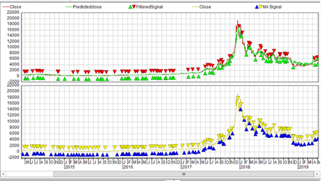
And the figure below shows other parameters for these two signals:
Observations
- Filtered Signal profitability is higher than Buy and Hold
- Filtered Signal profitability is higher than Simple MA Signal
- Number of trades reduces for Filtered Signal
- Percent win increases for Filtered Signal
- Sharpe ratio for Filtered Signal is higher than that of MA Signal
Approach-2
In this approach, for simulation of close on walk forward basis instead of using backpropagation, we used LSTM neural network. Below are four different simulations done:
Walk forward Simulations
In this approach we did four different walk forward simulations as described below:
Walk forward simulation using LSTM (1 hidden Layer) — Features Selected based on correlation >0.1 and <0.95
Walk forward simulation using LSTM (2 hidden Layer) — Features Selected based on correlation >0.1 and <0.95
Walk forward simulation using LSTM (1 Hidden Layer) — only All HODL Waves
Walk forward simulation using LSTM (2 Hidden Layer) — only All HODL Waves
The predicted close with 2 Hidden Layer and all hodl waves is much more stable than other cases. However, the differences between predicted and actual close are not significant except during major runups to ATHs. And that can help to get exit signals while entry signals are obtained by combining it with other existing models e.g. Stock flow model
Stock Flow Model
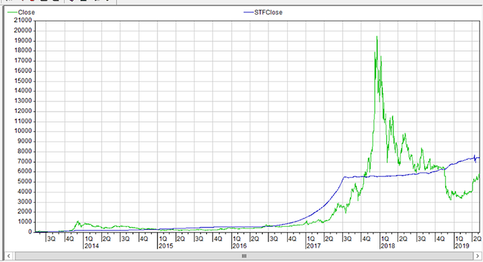
We computed close based on stock-to-flow model using the below expressions:
StockFlow= Annual Change in Stock/Current Stock
STFClose = 0.4*pow(StockFlow,3)
The resulting close is compared with actual close in The figure below:
Value Analysis
Below is the procedure used for value analysis of this approach:
- Design Two Trading Signals Using Simple Strategy based on Simple Moving Average (SMA)
- MA Signal with SMA2 (2 Sample) and SMA11 (11 Sample) for actual close
- Filtered Signal by combining
- MA Signal with SMA2 (2 Sample) for actual close and SMA11 (11 Sample) for predicted close
- Filter above signal such as buy only if actual close is below STFClose and sell only if actual close is above STFClose
- Trading Strategy
- Start Equity 100K
- Brokerage 0.075%
- Today’s Signal to be executed on next day ‘open price’
- Compare the equity gain of filtered signal with MA Signal
- Compare the equity gain of filtered signal with Buy and Hold
- Compare risk return parameters for above two signals
The figure below shows the comparison of two trading signals described above:
And figure below shows other parameters for these two signals:
Trading Strategy Results for All variations
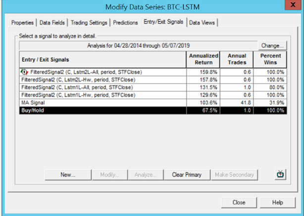
Observations
- Trading Signal outperforms buy/hold
- Trading Signal outperforms MA based Signal
- Sharpe ratio for Trading Signal is 1.89
- Number of Trades for Trading Signal are much less
- Percent win for Trading Signal is 80–100%
Approach-3
In this approach we try to use HODL waves with conventional indicators to derive a trading/investment strategy by combining MA signal for close and for hodl waves. The figure below shows the hold waves for bitcoin from sentiment database:
Value Analysis
Below is the procedure used for value analysis of this approach:
- Design Two Trading Signals Using Simple Strategy based on Simple Moving Average (SMA)
- MA Signal with SMA2 (2 Sample) and SMA11 (11 Sample) for actual close
- Filtered Signal by combining
- MA Crossing Signal with SMA2 (2 Sample) for actual close and SMA11 (11 Sample) for close
- Compute MA signal for HODL wave
- Take the trade only if both above signal have same signal
- Trading Strategy
- Start Equity 100K
- Brokerage 0.075%
- Today’s Signal to be executed on next day ‘open price’
- Compare the equity gain of filtered signal with MA Signal
- Compare the equity gain of filtered signal with Buy and Hold
- Compare risk return parameters for above two signals
The figure below shows all the trading signals for different HODL waves:
The figure below shows comparison of gain in equity between MA Signal and best HODL WAVE Trading Signal:
Figure below shows the comparison of signals from all the HODL waves:
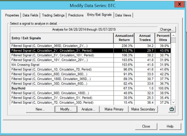
Observations
- Most Hodl Wave Trading Signals outperform buy/hold
- Some Hodl Wave Trading Signals outperform MA Signal
Approach-4
In approach-1 and 2 we tried to predict close price and then used the predicted price along with actual price to come up with a trading strategy. This approach is criticized as absolute values of close are not stationary and carry the memory which is leaked to neural network enabling large correlation between predicted close and actual close. Therefore, the economic literature suggest to use percent change or log returns as target output.
In this approach we will predict percent change of close for 7 days ahead on walk forward basis and use the predicted percent change of close to come up with a trading strategy. The selection of 7 days is at best arbitrary. The only thought process behind this number is that the next hold wave available after 1 day hodl wave is 7 day hodl wave. We could select 1 day percent change but that is expected to be more volatile than 7 day percent change.
Before doing the walk forward based simulation first we will do basic analysis to understand causality. First we remove highly correlated features (correlation>0.95) as described in approach-1. The remaining features are:
[‘BTC_hodl_waves.csv_circulation_2y’ ‘CostPerTransaction’
‘BTC_hodl_waves.csv_circulation_3y’
‘BTC_realized_value.csv_realized_value’ ‘Difficulty’
‘BTC_realized_cap.csv_realized_cap_180d’ ‘openPriceUsd’
‘BTC_hodl_waves.csv_circulation_365d’ ‘volume’
‘BTC_bounded_mvrv.csv_mvrv_1d’
‘BTC_active_coins.csv_% of coins active last 3 years’
‘BTC_hodl_waves.csv_circulation_10y’
‘BTC_active_coins.csv_% of coins active last 1 years’ ‘BlocksSize’
‘BTC_marketcaps.csv_circulation_1d’ ‘github_activity’ ‘AvgBlockSize’
‘transaction_volume’ ‘dev_activity’ ‘daily_active_addresses’
‘BTC_hodl_waves.csv_circulation_180d’ ‘Ntransactions’
‘MedianConfirmationTime’ ‘transactionfees’
‘BTC_hodl_waves.csv_circulation_60d’ ‘burn_rate’
‘BTC_hodl_waves.csv_circulation_30d’ ‘token_circulation’
‘BTC_mvrv_diff.csv_MVRV Long/Short Diff’ ‘BTC_bounded_mvrv.csv_mvrv_60d’
‘BTC_bounded_mvrv.csv_mvrv_180d’ ‘BTC_bounded_mvrv.csv_mvrv_30d’
‘mvrv_ratio’]
Then we carry out correlation analysis with absolute values of above selected features with true 7 days forward percent change of close to understand the causality. The figure below shows the correlation of selected features with 7 days forward percent change of close:
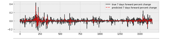
When these features are used to train and predict entire data range through a backpropagation neural network then we get results that are shown in The figure below:
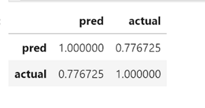
The correlation of predicted 7 days forward percent change with true 7 days forward percent change is shown in The figure below:
We also carry out correlation analysis of 1day backward percent change of above selected features with true 7 days forward percent change of close to understand the causality. The figure below shows the correlation of 1day backward percent change of above selected features with 7 days forward percent change of close:
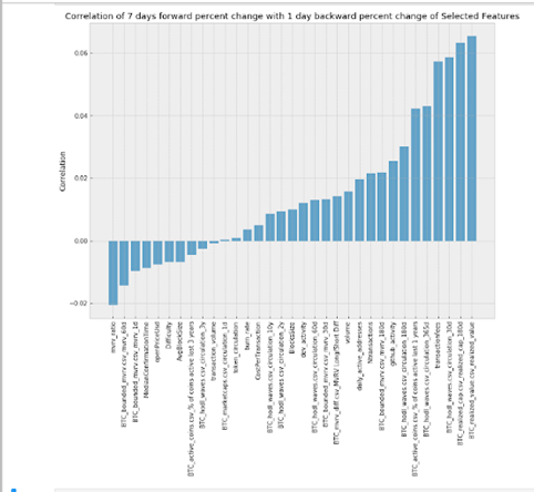
When the 1 day backward percent change of features are used to train and predict entire data range through a backpropagation neural network then we get results that are shown in The figure below;
The correlation of predicted 7 days forward percent change with true 7 days forward percent change is shown in The figure below:
It is obvious that while predicting 7 days forward percent change using 1 day backward percent change of features gives slightly better results than using absolute values of features.
Walk Forward Simulation
The above modelled 7 days forward percent change of close is not suitable to build a trading/investment strategy as in this case entire data was used to train and model in one go. So, to simulate the real-world scenario we will have to do this modelling in walk forward basis as described before. The 7 days forward percent change of close that is modelled through walk forward simulation can be the representative 7 days forward percent change of close that can be then used to build a trading strategy.
During simulation we found that using only HODL waves provides stable results than using all the features. Therefore, for walk forward simulation we used only HODL waves.
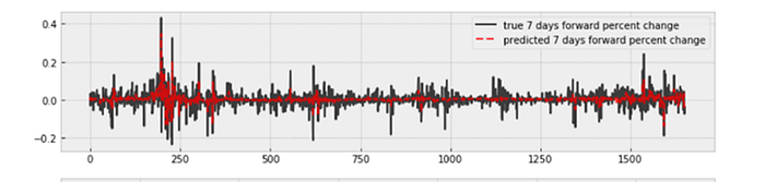
The figure below shows the comparison of true 7 days forward percent change of close with predicted 7 days forward percent change of close:
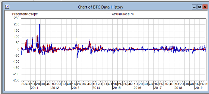
Correlation Analysis of true 7 days forward percent change of close with predicted 7 days forward percent change of close is shown below for different shifts.
Clearly the correlation analysis is low for no shift i.e. 0.2732 for walkforward based simulation than when entire data set was used in go i.e. 0.77. But this is the best that can be expected in real-world scenario.
Therefore, predicted percent change alone cannot be used to come up with trading signal. However, by combining it with conventional SMA crossing based signal could be useful.
Value Analysis
Below is the procedure used for value analysis of this approach:
- Design Two Trading Signals Using Simple Strategy based on Simple Moving Average (SMA)
- MA Signal with SMA2 (2 Sample) and SMA11 (11 Sample) for actual close
- Filtered Signal by combining
- MA Crossing Signal with SMA2 (2 Sample) and SMA11 (11 Sample) for actual close
- MA Crossing Signal with SMA2 (2 Sample) and SMA11 (11 Sample) for 7 days ahead predicted percent change of close
- Take the trade only if both above signal have same signal
- Trading Strategy
- Start Equity 100K
- Brokerage 0.075%
- Today’s Signal to be executed on next day ‘open price’
- Compare the equity gain of filtered signal with MA Signal
- Compare the equity gain of filtered signal with Buy and Hold
- Compare risk return parameters for above two signals
The figure below shows all the trading signals:
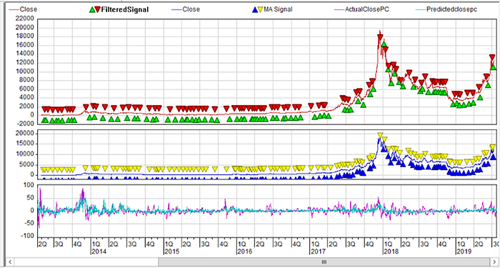
And figures below shows other parameters for these two signals:
Observations
Although results are better than buy and hold, the MA based strategy is superior to that of the approach-based signal in terms of overall equity gain. However, for percent wins strategy signal is better than that of MA Signal.
Approach-5
The predicted 7 days percent change has a correlation of 0.27 with true 7 days percent change. Using it as such has not produced results better than MA based signal. And on the other hand absolute close based approach-1 gave better results.
Which of the two approaches, absolute value based or percent change based, one should use is a typical dilemma in Fintech world while using AI and known as the Stationarity vs. Memory Dilemma. The dilemma is — returns are stationary however memory-less; and — prices have memory however they are non-stationary.
Therefore, we decided to merge the two approaches in our approach-5 as discussed below:
We accumulated the predicted 7 days percent change and plotted. Below are results:

And computed the correlation of actual close with accumulated predicted percent change and same are shown below:

The correlation analysis shows a correlation of 0.55. We are encouraged to use it as input to a backpropagation neural network to predict the close in walk forward mode as detailed below:
Walk forward Simulation
As described above the walk forward simulation is done to predict close while the input of the neural network was accumulated predicted percent change.
The predicted percent change, computed in approach-4, on walk forward basis satisfies stationarity requirement. And predicted close on walk forward basis using accumulated percent change satisfies memory requirement. So effectively in this approach we have tried to combine two different approaches in sequence that individually satisfy each requirement.
Value Analysis
Below is the procedure used for value analysis of this approach:
- Design Two Trading Signals Using Simple Strategy based on Simple Moving Average (SMA)
- MA Signal with SMA2 (2 Sample) and SMA11 (11 Sample) for actual close
- Filtered Signal by combining
- Bit complex
- Trading Strategy
- Start Equity 100K
- Brokerage 0.075%
- Today’s Signal to be executed on next day ‘open price’
- Compare the equity gain of filtered signal with MA Signal
- Compare the equity gain of filtered signal with Buy and Hold
- Compare risk return parameters for above two signals
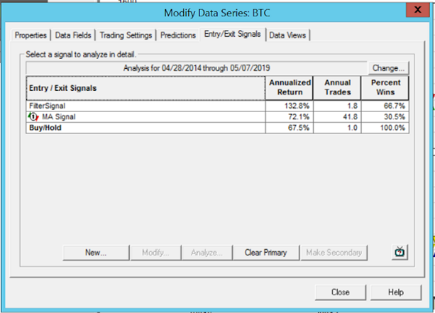
The figure below shows all the trading signals:

The figure belows shows additional analysis of these trading signals:

Observations
Below are observations for the results of this approach
- Win ratio >66%
- Returns better than MA based strategy
- Returns better than buy and hold
- Sharpe 1.68
- SO FAR THE BEST RESULTS BY ALL CRITERIA
All the Approaches in One Frame
The figure below shows a comparison of all the approaches in one frame
In approach-2 and approach-5 — we have successfully captured exit points just when prices start dropping from the ATH of that cycle and for all the cycles. This is in addition to successfully being able to enter the market near the bottom of the bear phase. We think that we have been able to achieve the objectives of the study.
Analysis for Ethereum
From the analysis of Bitcoin data and performance of various approaches — We decided to test approach-5 on Ethereum. Although both assets have different characteristics including maximum supply which is capped in case of bitcoin but not in case of Ethereum, yet it is good to test on Ethereum which will also act as complete blind test for the methodology.
The HODL waves for Ethereum are available in sentiment database. The figure below shows Ethereum hodl waves:
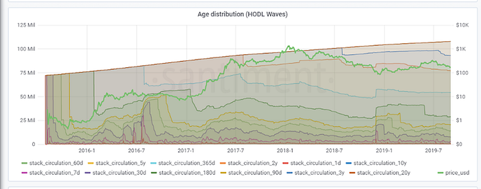
Data used for Ethereum is from 8 Aug-2015 to 17-Aug-2019.
Approach-5
As described in the case of bitcoin above, first we did walk forward simulation for 7 days forward percent change using only HODL waves as input.
Walk forward simulation for 7 days forward percent change
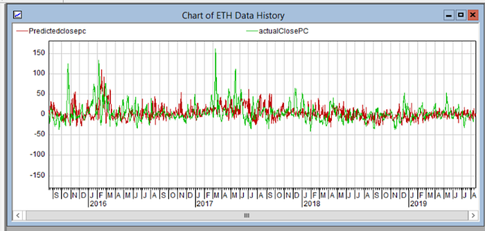
For ETH we used exactly same procedure as described for approach#5 in case of BTC. The figure below shows the comparison of true 7 days forward percent change of close with predicted 7 days forward percent change of close:
Correlation Analysis of true 7 days forward percent change of close with predicted 7 days forward percent change of close is shown below for different shifts.
Clearly the correlation is very low for no shift i.e. 0.059. But this is the best that can be expected in real-world scenario. Therefore, predicted percent change alone cannot be used to come up with trading signal.
So. as discussed in the case of Bitcoin — we accumulated the predicted 7 days percent change and plotted. Below are results:
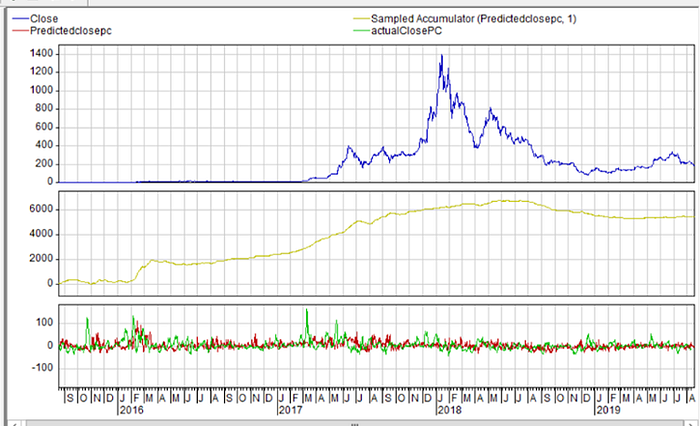
And computed the correlation of actual close with accumulated predicted percent change and same are shown below:
The correlation analysis shows a correlation of 0.72. We are encouraged to use it as input to a backpropagation neural network to predict the close in walk forward mode as detailed below:
Walk forward Simulation for close
As described above the walk forward simulation is done to predict close while the input of the neural network was accumulated predicted percent change. The results are shown in the below figure:
Value Analysis
Below is the procedure used for value analysis of this approach:
- Design Two Trading Signals Using Simple Strategy based on Simple Moving Average (SMA)
- MA Signal with SMA2 (2 Sample) and SMA11 (11 Sample) for actual close
- Filtered Signal by combining
- Bit complex
- Trading Strategy
- Start Equity 100K
- Brokerage 0.075%
- Today’s Signal to be executed on next day ‘open price’
- Compare the equity gain of filtered signal with MA Signal
- Compare the equity gain of filtered signal with Buy and Hold
- Compare risk return parameters for above two signals
The figure below shows all the trading signals:
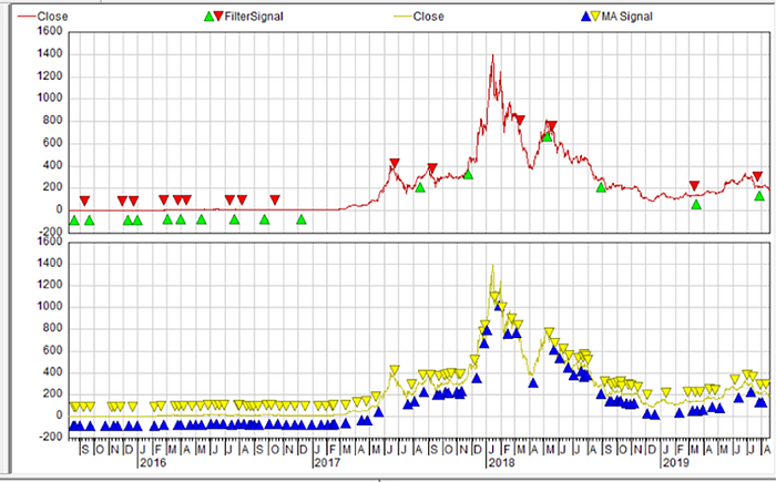
The figure belows show additional analysis of these trading signals:
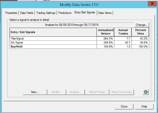
Observations
Below are observations for the results of this approach
- Win ratio >45%
- Returns better than MA based strategy
- Returns better than buy and hold
- Sharpe 1.68
- Blind test is successful
Impact on Profitability due to bid/ask Spread and Slippage
In all the simulations above only a brokerage of 0.075% is assumed. However, in real case there will be an adverse effect on profitability due to bid/ask spread and slippage. When number of trades are more for a strategy then these effects can not be ignored and must be included. If we add conservative bid/ask spread of 0.1% and slippage of 0.1% on top of 0.075% brokerage — then below are the results of approach#5 for bitcoin and ethereum:
Bitcoin Results
Ethereum Results
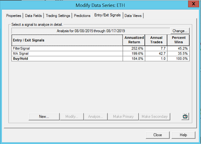
It is obvious that any strategy that generates a lot of trades — is bound to produce poorer results because prediction accuracy is going to be low for high frequency trading strategy. On the other hand, even with moderate prediction accuracy a strategy, that generates less trades with large profit per trade, is expected to produce reasonably good results.
Conclusions and Recommendations
Below are our conclusions and recommendations from the study:
Conclusions
- Most existing models give good entry points after major bear phase
- But all of them fail to provide good exit points
- There is very good causality between many features that we had and close
- The prediction of actual close using backpropagation as well as LSTM neural network is good and helps pick major undervalued zones.
- There is no significant causality between all the features that we had and percent change of close
- Prediction of percent change of close using RNN is not very satisfactory which is expected as there is a lack of causality between input and output.
- HODL waves are much more stable features than other features. That is the reason neural network based prediction of actual close as well as percent change of close is more stable when only HODL waves are used as input to neural networks
- The predicted percent change, computed in approach-4, on walk forward basis satisfies stationarity requirement. And predicted close, computed in approach#5, using accumulated percent change satisfies memory requirement. So effectively in approach#5 we have tried to combine two different approaches in sequence that individually satisfy requirement of stationarity and memory.
- Many other criticisms of neural network based approach, like randomization of initial state, over training, selection of training and validation datasets, selection of network parameters etc, are taken care of as we do everything on walk forward basis. So if there is a sub optimum training and prediction due to any of the neural network related issues then as we are doing afresh for each sample -the potential damage on our ability to train and predict will be temporary on few samples. And we do see it in our predicted values as some values jump abnormally up or down but soon starts following the overall trend.
- We have developed and tested five different approaches.
- All the approaches have produced better results than buy and hold
- All the approaches have produced better results than simple MA based strategy except approach#4.
- Approach#5 is preferred approach as it also addresses the dilemma of stationarity vs memory and results are also good
- Approach#5 also help us consistently pick reasonably good exit/short point after ATH of each bull/bear cycle.
Recommendations
In order to reduce volatility of returns below are our recommendations:
- Use 50% of the account value to trade using these signals. We used 100% of the account value.
- Generate trading signals using approach#5 on other reasonably liquid, top 20/30, assets and include them in the portfolio.
- We used simple SMA based strategy to establish value of data and methodology. We expect that results can be improved with more advanced strategies.
- Deploy hedging strategies
- Although we tried our best to include all relevant features into our study yet it would be unfair to say that we were able to study and extract all the value hidden in data available in Santiment database. We will keep working on newer ideas and share any new findings with the community.
Abbreviations
ATH — All time high
SMA — Simple Moving Average
MA — Moving Average
HODL — HOLD equivalent in Crypto
LSTM — Long Short Term Memory
RNN — Recurrent Neural Network
Acknowledgement
This is a collaborative work between Santiment and ShilazTech Teams over 3–4 months period. We have had very constructive discussions and feedbacks from many experts. Personally I would like to extend my thanks to Jan Smirny , Nemanja Cerovac, Tzanko Matev, and Dindustries for their invaluable inputs. I would also like to thank Maksim Balashevich, founder Santiment, for sponsoring the study.