Linear Regression

Finding the best-fitting straight line through the points of a data set.

Linear Regression is the oldest, simple and widely used supervised machine learning algorithm for regression problems.

• [Linear approach to modelling the relationship between a dependent variable and one or more independent variables.]

It’s a method to predict a target variable by fitting the best linear relationship between the dependent and independent variable.

• Linear Regression models the relationship between a dependent variable (y) and one or more independent variables (X) using a best fit straight line (also known as regression line). The dependent variable is continuous. The independent variable(s) can be continuous or discrete, and the nature of the relationship is linear.
• Linear relationships can either be positive or negative. A positive relationship between two variables basically means that an increase in the value of one variable also implies an increase in the value of the other variable. A negative relationship between two variables means that an increase in the value of one variable implies a decrease in the value of the other variable. (Correlation helps determine this relationship between variables)

Simple linear regression is an approach for predicting a quantitative response Y on the basis of a single predictor variable X. It assumes that there is approximately a linear relationship between X and Y .

The picture 1. below, borrowed from the first chapter of this stunning machine learning series, shows the housing prices from a fantasy country somewhere in the world. You are collecting real-estate information because you want to predict the house prices given, say, the size in square feet.

Given your input data, how can you predict any house price outside your initial data set?

• For example, how much a 1100 square feet house is worth?

Linear regression will help answering that question: you shrink your data into a line (the dotted one in the picture above), with a corresponding mathematical equation, f. If you know the equation of that line, you can find any output (y) given any input (X).

Terminology and Terms

When you gathered your initial data, you actually created the so-called training set, which is the set of housing prices. The algorithm’s job is to learn from those data to predict prices of new houses. You are using input data to train the program, that’s where the name comes from.

• The number of training examples, are noted as m; the input variable x is the single house size and y is the output variable, namely the price.

The list (x,y) denotes a single, generic training example, while (x^(i), y^(i)) represents a specific training example.

So if I write (x^(2), y^(2)) I’m referring to the second row in the table above, where x(2) = 1510 and y(2) = 310,000.

The training set of housing prices is fed into the learning algorithm. Its main job is to produce a function, which by convention is called h (for hypothesis). You then use that hypothesis function to output the estimate house price y, by giving it the size of a house in input x.

y = h(X)

More Understanding or Linear Regression problem

If we know there exists a linear relationship between the independent variable, and the dependent variable:

we can use linear regression to this kind of data. However, the goal is to find the best fitting line parameters that best suits our data.

Hypothesis function

Hypothesis function is represented as:

θ’s are the parameters of the function. Usually the θ subscript gets dropped and the hypothesis function is simply written as h(x).

• That formula might look scary, but if you think about it, it’s nothing fancier than the traditional equation of a line, except that we use θ’s.

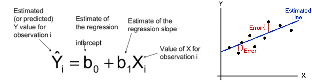
Mathematically, the line representing a simple linear regression is expressed through a basic equation:

• Together 𝛽0 and 𝛽1 known as the model coefficients or parameters.

In fact the hypothesis function is just the equation of the line.

In our humble hypothesis function there is only one variable, that is x. For this reason our task is often called linear regression with one variable. Experts call it also uni-variate linear regression, where uni-variate means “one variable”.

Understanding slope and intercept

Cost function

Well, at this point we know that there’s a hypothesis function to be found. More precisely we have to find the optimal parameters (θ values) so that the hypothesis function best fits the training data.

If you recall how the equation of a line works, those two parameters control the slope and the height of the line.

We definitely want a best fit line that fits our data. So how to find optimal θ values?

You certainly recall that in our training set we have several examples where we know the size of the house x and the actual price of the house y. We know those prices and sizes because we previously took a survey for those data.

So the idea in a nutshell: let’s try to choose the hypothesis function parameters (θ values) so that, at least in the existing training set, given the x as input parameter to the hypothesis function we make reasonably accurate predictions for the y values. Once we are satisfied, we can use the hypothesis function with its pretty parameters to make predictions on new input data.

Residuals

Residual Sum of Squares (RSS)

Whichever the line that gives low residual error for all data points, we chose that line as best fitting line.

• The squaring is done so negative values do not cancel positive values.

Problem: RSS value will change if we change kind of scale of our features. (gm → Kg ). Try to calculate RSS by changing the scale of values.

Total Sum of Squares (TSS)

One way to handle this is, TSS (Total Sum of squares). In this we calculate mean and take difference between actual and mean value.

R² (Coefficient of Determination)

We always look for R² value to be high.

R² is a statistic that will give some information about the goodness of fit of a model.

In regression, the R² coefficient of determination is a statistical measure of how well the regression predictions approximate the real data points. An R² of 1 indicates that the regression predictions perfectly fit the data.

R² visual representation:

from sklearn.metrics import r2_score
print("R2 score : %.2f" % r2_score(ytest, preds))

Mean Squared Error (MSE)

It measures how close a fitted line is to the data points.

• The smaller the MSE, the closer the fit is to the data. Actually there are many other functions that work well for such task, but the MSE is the most commonly used one for regression problems.

If I plug our data into the MSE function, our final formula looks like that:

• For every data point, you take the distance vertically from the point to the corresponding ‘y’ value on the curve fit (the error/residual), and square the value. Then you add up all those values for all data points, and, divide by the number of points. The squaring is done so negative values do not cancel positive values.

Why divide by 2m ?

• The only reason some authors like to include it is because when you take the derivative with respect to x, the 2 goes away.

By convention we would define a cost function (aka loss function), J , that is just the above equation written more compact:

Now, we want to find good values of θ, so good that the above cost function can produce the best possible values, namely the smallest ones (because small values mean less errors). This is an optimization problem: the problem of finding the best solution from all feasible solutions.

— — For a line passing through origin, θzero = 0. The cost function, J will be:

MSE and RSME

The Mean Squared Error (MSE) is a measure of how close a fitted line is to data points. The smaller the Mean Squared Error, the closer the fit is to the data. The MSE has the units squared of whatever is plotted on the vertical axis.

Another quantity that we calculate is the Root Mean Squared Error (RMSE). It is just the square root of the mean square error.

That is probably the most easily interpreted statistic, since it has the same units as the quantity plotted on the vertical axis.

Key point: The RMSE is thus the distance, on average, of a data point from the fitted line, measured along a vertical line.

from sklearn.metrics import mean_squared_error
print("Mean squared error: %.2f" % mean_squared_error(ytest, preds))
print('RMSE :', np.sqrt(mean_squared_error(y_test, preds)))

Optimization Algorithm

The goal is to have the optimal θ values, that gives low RMSE value. But the question, how to calculate optimal θ values? We use a learning technique to find a good set of coefficient values. Before that, let’s try to visualize cost function w.r.t feature variables.

Visualizing cost function

If we have only 1 feature, then it will 2-D plot to visualize cost function w.r.t feature variable.

In the real world, 3-dimensional (and even more!) cost functions are quite common. Fortunately there are some neat ways to visualize them without losing too much information and mental sanity.

Here, we have plotted cost function w.r.t 2 feature variables.

It looks like a cup and the optimization problem turns to be finding the best θ values that results in lowest point on the bottom edge.

Sometimes, when the picture becomes too messy, it’s common to switch to another representation: the contour plot. A contour plot is a graphical technique for representing a 3-dimensional surface by plotting constant horizontal slices, called contours, on a 2-dimensional format.

• What we actually want is our program to find optimal ‘θ’ values that minimize the cost function.

To update θ values in order to reduce Cost function (minimizing RMSE value) and achieving the best fit line, the model uses Gradient Descent.

— — The idea is to start with random θ values and then iteratively updating the values, reaching minimum cost.

Gradient Descent algorithm

How to find the minimum of a function using an iterative algorithm.

Optimization is a big part of machine learning. Almost every machine learning algorithm has an optimization algorithm at it’s core.

Gradient Descent is one of the most popular and widely used optimization algorithm.

• Given a machine learning model with parameters (weights and biases) and a cost function(or loss function), to evaluate how good a particular model is, our learning problem reduces to that of finding a good set of weights/parameters for our model which minimizes the cost function.

Learning a linear regression model means estimating the values of the coefficients used in the representation with the data that we have available.

Theory: Given a function defined by a set of parameters, gradient descent starts with an initial set of parameter values and iteratively moves toward a set of parameter values that minimize the function. This iterative minimization is achieved using calculus, taking steps in the negative direction of the function gradient.

Intuition

Imagine you’re blind folded in a rough terrain, and your objective is to reach the lowest altitude. One of the simplest strategies you can use, is to feel the ground in every direction, and take a step in the direction where the ground is descending the fastest. If you keep repeating this process, you might end up at the lake, or even better, somewhere in the huge valley.

The rough terrain is analogous to the cost function(or loss function). Minimizing the cost function is analogous to trying to reach lower altitudes. You are blind folded, since we don’t have the luxury of evaluating (seeing) the value of the function for every possible set of parameters. Feeling the slope of the terrain around you is analogous to calculating the gradient, and taking a step is analogous to one iteration of update to the parameters.

Gradient descent is an iterative method.

Multiple Linear Regression

So far, we looked at linear regression based on a single variable, meaning we had a single input feature x (the size of the house in the house pricing problem) that I used to predict the output y (the price of the house).

I eventually ended up with a hypothesis function for such problem:

Now, we will try to understand the more powerful version that works with multiple variables called multivariate linear regression, where the term multivariate is a fancy word for more than one variable.

The housing prediction problem with multiple features

You surely need more than one feature in order to better predict the price of a house, like for example the number of rooms, the number of floors, the age of the house itself and so on. Those are your new input features xx. Being more than one, we need to update the notation a little bit.

The hypothesis function has to be updated in order to work with multiple inputs. It’s going to be:

The magic is going to happen, thanks to the trick: any linear algebra wizard will now recognize the formula above as the inner product between two vectors.

By definition of the inner product, the first argument (θ) must be a row vector. However our θ is a column vector. That’s not a problem: just transpose it, that is make it a row (lay it down).

This notation will make the implementation way easier: computing the hypothesis function is now just a matter of an inner product between two vectors.

I’ve updated the hypothesis function to work with multiple input parameters. Both the gradient descent function and the cost function need some tweaks as well.

Preparing Data for Linear Regression

There is a lot of literature on how your data must be structured to make best use of the model.

• Linear Assumption: Linear regression assumes that the relationship between your input and output is linear. It does not support anything else. This may be obvious, but it is good to remember when you have a lot of attributes. You may need to transform data to make the relationship linear (e.g. log transform for an exponential relationship)
• Remove Noise: Linear regression assumes that your input and output variables are not noisy. Consider using data cleaning operations that let you better expose and clarify the signal in your data. This is most important for the output variable and you want to remove outliers in the output variable (y) if possible.
• Remove Collinearity: Linear regression will overfit your data when you have highly correlated input variables. Consider calculating pairwise correlations for your input data and removing the most correlated.
• Gaussian Distributions: Linear regression will make more reliable predictions if your input and output variables have a Gaussian distribution. You may get some benefit using transforms (e.g. log or BoxCox transform) on your variables to make their distribution more
  Gaussian looking.
• Rescale Inputs: Linear regression will often make more reliable predictions if you rescale input variables using standardization or normalization.
• Both input and output values are numeric.

SciKit-learn LinearRegression class

From the implementation point of view, this is just plain Ordinary Least Squares wrapped as a predictor object.

sklearn.linear_model.LinearRegression - scikit-learn 0.20.2 documentation

# Code source: Jaques Grobler
# License: BSD 3 clause


import matplotlib.pyplot as plt
import numpy as np
from sklearn import datasets, linear_model
from sklearn.metrics import mean_squared_error, r2_score

# Load the diabetes dataset
diabetes = datasets.load_diabetes()


# Use only one feature
diabetes_X = diabetes.data[:, np.newaxis, 2]

# Split the data into training/testing sets
diabetes_X_train = diabetes_X[:-20]
diabetes_X_test = diabetes_X[-20:]

# Split the targets into training/testing sets
diabetes_y_train = diabetes.target[:-20]
diabetes_y_test = diabetes.target[-20:]

# Create linear regression object
regr = linear_model.LinearRegression()

# Train the model using the training sets
regr.fit(diabetes_X_train, diabetes_y_train)

# Make predictions using the testing set
diabetes_y_pred = regr.predict(diabetes_X_test)

# The coefficients
print('Coefficients: \n', regr.coef_)
# The intercept
print('Intercept: \n', reg.intercept_)
# The mean squared error
print("Mean squared error: %.2f"
      % mean_squared_error(diabetes_y_test, diabetes_y_pred))
# Explained variance score: 1 is perfect prediction
print('Variance score: %.2f' % r2_score(diabetes_y_test, diabetes_y_pred))

# Plot outputs
plt.scatter(diabetes_X_test, diabetes_y_test,  color='black')
plt.plot(diabetes_X_test, diabetes_y_pred, color='blue', linewidth=3)

plt.xticks(())
plt.yticks(())

plt.show()

Sources

Internal pointers site
Gradient Descent algorithm