Simple Linear Regression Using Example.

In this piece, I’ll go through what simple linear regression is and how to use it on a dataset in depth.

8 min readMar 11, 2022

The following topics are covered in this tutorial:

what is Linear Regression?
Types of Linear Regression.
Linear Regression assumptions.
Correlation coefficient (r).
Coefficient of determination(R-squared ).
Residuals.
Lost/Cost Function.
Residual analysis.
Applying Linear Regression using Python.

What is Linear Regression?

We can describe linear regression as a form of predictive modeling technique that investigates the relationship between a dependent and independent variable.

**Linear Regression** [Image by Author (created using Canva)]

For example, if I look at an employee’s experience and salary, we can see that there is a linear relationship between the two. More the experience a person has, the greater their salary, and vice versa.

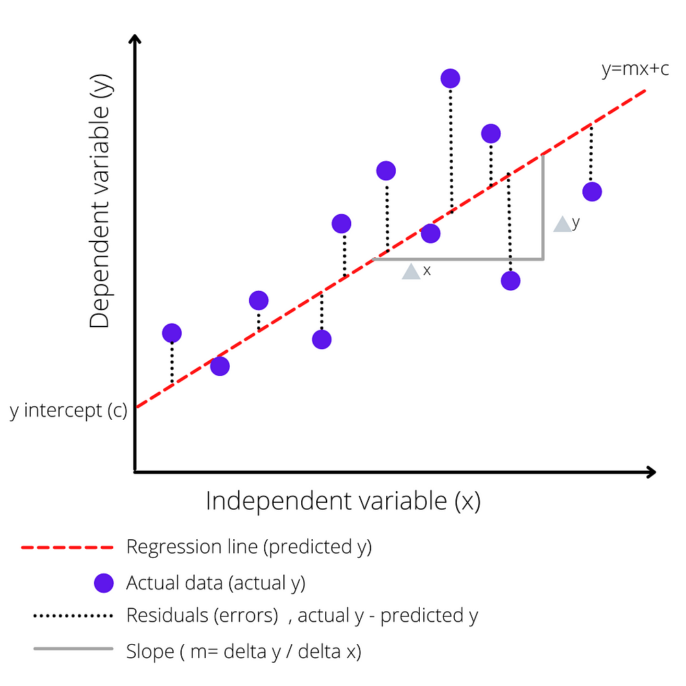
From the above graph, we can see that in linear regression we take the independent variable in the x-axis and dependent variable in the y-axis, and we try to fit the best line which has minimum error between actual and predicted value.

The following is a simple linear regression equation:

**Linear Regression Equation** [Image by Author(created using LaTex)]

The graph of a regression equation is a straight line.
c is the y-intercept of the regression line.
m is the slope of the regression line.
E(y) is the expected value of y for the given x value.

Types of Linear Regression.

Simple linear regression: In simple linear regression we have one independent variable(x) and one dependent variable(y), for that, we have to fit the best fit line.

Equation of a simple linear regression can be written as, Expected(y)=mx+c

2. Multiple linear regression: In multiple linear regression we have one dependent variable(y) and more than one independent variable(x), using these multiple variables we have to find a good relationship between these variables.

Equation of a Multiple linear regression can be written as, Expected(y) =c+ m1x1+m2x2+…….+mnxn .

Linear Regression assumptions.

A linear relationship between x and y variables.
There should be no or little multicollinearity.
Residuals should be independent of each other.
Residuals should be normally distributed with a mean of 0.
The assumption of homoscedasticity(“same variance”) is central to the linear regression model.

Correlation coefficient (r).

We use the Correlation coefficient (r) to describe the strength and direction of the relationship between independent and dependent variables.

**Correlation coefficient** [Image by Author (created using Canva)]

If we observe figure a, we can see a complete negative relationship between x and y variables, this is a condition when one of the variables increases and the other variable is depressing, this is a perfect negative linear relationship.
If we observe figure b, we can observe, r is varying between -1 and 0.
In figure c, we can observe r=0 which means there is no relationship between x and y variables.
In figure d, we can observe positive relation between x and y variables. Here we can see as one variable increases another one also increases.
In figure e, we can observe the perfect positive linear relationship between x and y variables.
Correlation coefficient (r) varies between -1 to +1.

Coefficient of determination(R-squared )

R-squared value explains the variability of y with respect to x.
R-squared value varies between 0 to 1(0 to 100%).
R-squared value is closer to 0 means the regression relationship is very low.
R-squared value is closer to 1 means the regression relationship is very strong.

Residuals.

If we observe a linear regression image we can say residuals are nothing but the difference between an actual dependent variable and a predicted dependent variable.

Lost/Cost Function.

To know how good or bad our model is performing we calculate the loss function. Using actual value and predicted value we calculate the loss function. In general, in linear regression, we use the ordinary least square method, mean squared error(MSE), root mean squared error (RMSE).

Residual analysis.

Residual analysis is the primary tool for determining whether the assumption made about the model is appropriate or not.

Residual analysis is based on examination of graphical plots:

A plot of residuals against values of the independent variable(x).
A plot of the residuals against predicted values of the dependent variable.
A standardized residual plot.
A normal probability plot.

Applying Linear Regression using Python.

In this example I am using a dataset that has two columns, one is years of experience and another one is salary. This is not a real-world dataset, it’s just a dummy dataset, using this dummy dataset I am going to perform simple linear regression.

I have downloaded this dataset from Kaggle, you can find it here.

We all know our salary depends on the number of years of experience we have, so in this dataset salary is a dependent variable(y) and years of experience is an independent variable(x).

I am running this code on Jupyter notebook in a Jovian. The link to this notebook is here.

First we have to import all the depending libraries to perform simple linear regression.

import numpy as np
import pandas as pd
import statsmodels.api as sm
from statsmodels.formula.api import ols
from bioinfokit import visuz
from bioinfokit.analys import stat, get_data
import seaborn as sns
import matplotlib.pyplot as plt
%matplotlib inline
import warnings
warnings.filterwarnings('ignore')

After importing all the necessary library ,we have to import out dataset.

data=pd.read_csv('Salary_Data.csv')

After importing datset,I am going to plot the scatter plot between dependent variable(salary) and independent variable (experience).

x=data['YearsExperience']
y=data['Salary']
plt.scatter(x,y)
plt.xlabel("YearsExperience")
plt.ylabel("Salary")
plt.title("Linear Regression plot")
plt.show()

Plot created using matplotlib[Image by Author]

here, in the above graph, we can see the positive relationship between dependent and independent variables.

Now,I will perform linear regression using ordinary least square method.

linear_regression=ols(formula="Salary~YearsExperience",data=data)
model=linear_regression.fit()
print(model.summary())OLS Regression Results                             ============================================================================== Dep. Variable:                 Salary   R-squared:                       0.957 Model:                            OLS   Adj. R-squared:                  0.955 Method:                 Least Squares   F-statistic:                     622.5 Date:                Fri, 04 Mar 2022   Prob (F-statistic):           1.14e-20 Time:                        14:55:10   Log-Likelihood:                -301.44 No. Observations:                  30   AIC:                             606.9 Df Residuals:                      28   BIC:                             609.7 Df Model:                           1                                          Covariance Type:            nonrobust                                          ===================================================================================                       coef    std err          t      P>|t|      [0.025      0.975] ----------------------------------------------------------------------------------- Intercept        2.579e+04   2273.053     11.347      0.000    2.11e+04    3.04e+04 YearsExperience  9449.9623    378.755     24.950      0.000    8674.119    1.02e+04 ============================================================================== Omnibus:                        2.140   Durbin-Watson:                   1.648 Prob(Omnibus):                  0.343   Jarque-Bera (JB):                1.569 Skew:                           0.363   Prob(JB):                        0.456 Kurtosis:                       2.147   Cond. No.                         13.2 ==============================================================================  Notes: [1] Standard Errors assume that the covariance matrix of the errors is correctly specified.

The regression line equation is , y =2.579e+04 + (9.449.9626 * YearExperience). This equation will help us to calculate salary for the given years of experience.
The y-intercept(c) is 25790 represents the value of y when x=0, which means even when an employee has 0 years of experience that person will be paid 25,790.
The slope(m) is 9.449.9626 representing the change in per unit area of y to the change in a unit area of x. It means salary will increase by 9449.9626 with each unit increase in the experience.
coefficient of determination (R-squared) is .957(95.7%), the regression relationship is very strong. 95.7% of the variability in the salary can be explained by independent variable years of experience.

Using above regression equation I am calculating the new salary value(yhat),for the same independent variable x.

data['yhat']=model.predict(x)
data.head(5)

Screenshot of a notebook [Image by Author]

yhat is the new predicted salary for the years of experience.

Visualizing Regression line.

visuz.stat.regplot(df=data, x='YearsExperience', 
                   y='Salary', yhat='yhat',show=True)

In this step we are calculating loss function.

residual= stat()
residual.reg_metric(y=np.array(y),
                    yhat=np.array(model.predict(x)),
                    resid=np.array(model.resid))
residual.reg_metric_df.head(2)

Root Mean Square Error(RMSE) means, on average, each element in the predicted salary(yhat) differs from the actual salary by 5592.
Mean Squared Error(MSE) means, on average, each element in the predicted salary(yhat) differs from the actual salary by the square root of the loss 3.127095e+07, which is also 5592.
The result is called the loss function because it indicates how bad the model is at predicting the target variables. It represents information loss in the model: the lower the loss, the better the model.

Now we will perform residual analysis to check the assumptions we made about the model.

sns.residplot(data['YearsExperience'],data['residual'],color='g');

The above graph is a plot of residuals against values of the independent variable(x).
Here, we can observe that data is almost equally distributed around residual=0, from this we can say it meets the assumption we made that linearity between x and y and Residuals should be normally distributed with a mean of 0.

sns.residplot(data['yhat'],data['residual'],color='g');

The above graph is a plot of the residuals against predicted values of the dependent variable (yhat).
Here, we can observe that data is almost equally distributed around residual=0, from this we can say it meets the assumption we made that linearity between x and y and Residuals should be normally distributed with a mean of 0.

influence=model.get_influence()
residual_salary=influence.resid_studentized_external
sns.residplot(data['Salary'],residual_salary,color='g');

The above graph represents a standardized residual plot.
The residuals are between the range of +2 to -2, which suggests that it meets the assumption of linearity.

sm.qqplot(data['standardized_residual'], line='45')
plt.xlabel("Theoretical Quantiles")
plt.ylabel("Standardized Residuals")
plt.title('qq-plot -residuals of ols fit')
plt.show()

The above graph represents a normal probability plot.
From the above plot, we can observe that all the blue dots are near the red line, which suggests that residuals are normally distributed.

Summary

In this piece, we discussed what is regression, types of regression, what are the assumptions we make while performing regression, different metrics to measure the strength and direction of the regression line, we learned how to perform linear regression using OLS, and different loss functions and also we have seen how to perform residual analysis.

In the upcoming post, even I’ll further discuss the remaining left out topics and also how to perform regression using scikit-learn and also using PyTorch.