P-value, Level of significance, Hypothesis testing, Z scores, Type I / II errors

15 min readApr 26, 2022

This article is about P-value and all the topics required to better understand P-value.
The idea of article is to introduce all the pre-requisites and then finally introduce P-value. Hence, the article will talk about a lot of topics before reaching to a conclusion. I hope I won’t leave any jargon for you to figure out from google.

Density Curve

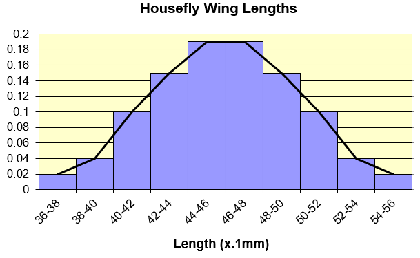
Let’s start off with density curves. Let’s assume we have a dataset that can be represented via a normal distribution as shown below.

We can convert this normal frequency distribution into relative frequency distribution as shown below.

fig 2: relative frequency based distribution

The curve that we draw on top of relative frequency distribution is the density curve as shown in fig 3. Total area under a density curve is equal to 1. This is because density curve is made on top of relative frequency distribution curve wherein total of data points is equal to 1 (0.02 + 0.04 + 0.1 + 0.15 + 0.19 + 0.19 + 0.15 + 0.1 + 0.04 + 0.02) as shown in fig 2.

Density curve in above fig 3 does not look smooth enough but if we have a dataset large enough, the curve will be smooth based on central limit theorem. I have given an example below for the same.

Some instances of central limit theorem are shared in the article that I had written on chi-squared test. Please search central limit theorem in the chi-squared article to find its usage.

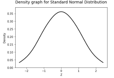
Now, since we have density curve as shown in fig 3, we need to convert the normally distributed data into standard normal distribution. This can be done using a simple formula. We did this using python code and the output along with code is shown below.

fig 5: Standard normal distribution of dataset via python code

Quick facts about Standard normal distribution and Z score below:

We know that standard normal distribution has a mean of 0 and SD of 1.
X axis of the standard normal distribution is called as Z score.
Z score measures the distance of an observed value from mean of standard normal distribution.
Z score is measured in units of standard deviations.
Z score is 0 at the mean of standard normal distribution.

Z Score table

A glimpse of Z score table present in appendix section of major statistics books is shown below for reference.

I have given below couple of examples to understand how is a Z score used.

Example 1: 50 randomly selected volunteers took an IQ test. Helen, one of the volunteers, scored 74 (X) from maximum possible 120 points. The average score was 62 (µ) and the standard deviation was 11 (σ). How well did she do on the test compared to other volunteers?

First, we know what marks follow a standard distribution just like height, weight etc. Hence, we can take this as a Z-score standard normal distribution problem.

In order to find out how well Helen did, her IQ test points need to be converted to a standardized z-score

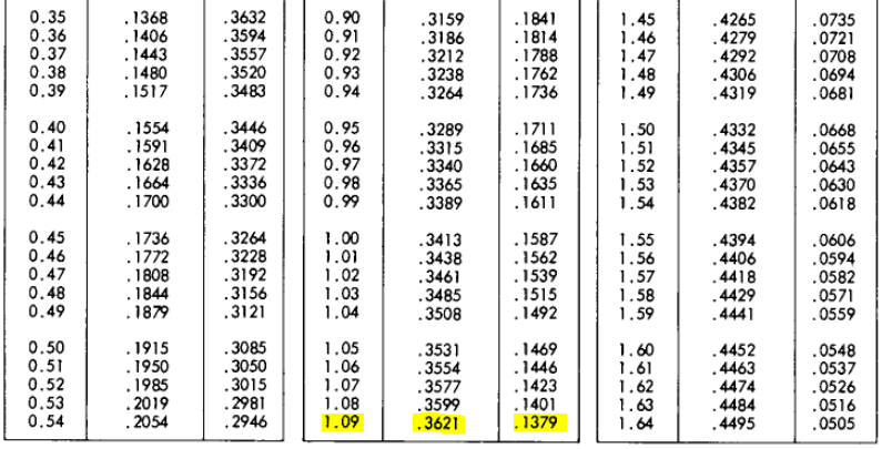
(74–62) / 11 = 1.09090909 ~ 1.09

After calculating the standardized score, we need to look up the area (same as probability) using the z-table. First, we find the first two digits on the left side of the z-table. In this case it is 1.0. Then, we look up a remaining number across the table (on the top) which is 0.09 in our example. The corresponding area is 0.8621 which translates into 86.21%.

fig 7: Z score table with highlighted values

The area that we looked up in the z-table suggests that Helen received a better score than 86% of the volunteers who took the IQ test. If you would like to know an exact number of people who Helen outperformed at the test, then just multiply 50 (remember that’s how many people took the test) by 0.8621 which is 43.1. As there are no partial human beings, we just round the number to 43. Helen did better than other 43 test takers.

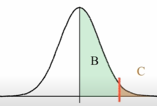
Now, there is another version of z score table which is seen below. This table refers to image in figure 10.The output required in Example 1 can be derived from this z score table as well.

fig 9: table for area under normal curve.

The output of Example 1–1.09 can be traced in this Z score table as shown below in figure 11. Value of B is 0.361 and value of C is 0.1379. Now, since Z score graph is symmetric, the area for left negative half of the graph is (B+C). The meaning of B and C can be understood from fig 10.

What percentage of people did Helen did better?

(B+C) + B = (0.361 + 0.1379) + 0.361 = 0.8621 ~ 86.21%

fig 11: area under normal curve: output of example 1.

Before proceeding further with understanding P-value, let’s first understand another concept of Hypothesis testing.

Hypothesis Testing

Hypothesis testing means “a supposition made on the basis of limited evidence as a starting point for further investigation”.

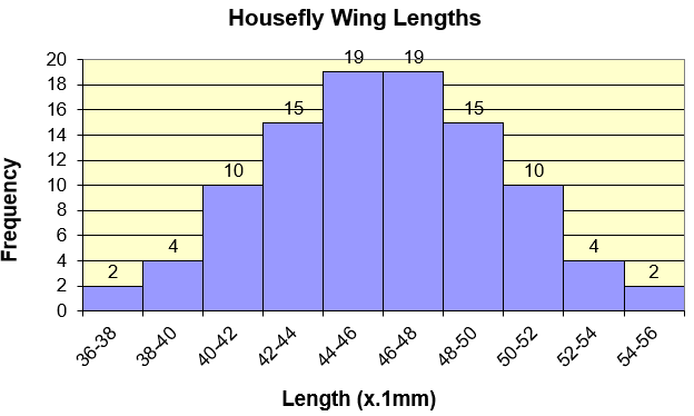
When we do an experiment in statistics, there is a possibility of an outcome in either directions. Let’s say we have the same data of housefly as shown in fig 1.

Scientists are trying to understand if there is a widespread disease in houseflies in recent times which is holding their growing capability and affecting their wing length. Scientist conducts an experiment on a newly picked housefly with an assumption that there is no new disease in the housefly and the newly picked housefly will have more or less similar wing length to other housefly’s wing length.

Post the experiment, the wing length came out extremely low and falls in the lowest most left part of normal distribution of the housefly wing length’s dataset as shown in fig 1.

Now, the same experiment description can be written in terms of hypothesis test.

Null hypothesis: H0: The assumption with which the test is conducted is basis for Null hypothesis. “The newly picked housefly’s wing length is no different from other housefly’s wing length.”

Alternative hypothesis: H1: HA: Alternate hypothesis is what scientist wants to prove. “The newly picked housefly’s wing length is extremely different from the other housefly’s wing length.”

Outcomes of hypothesis testing

The outcome of the test is based on a probability. This is because testing with a single observation or even few more samples won’t be sufficient to make concrete conclusions on the entire population of housefly’s wing lengths. There are two possible outcomes of a Hypothesis test that are explained below.

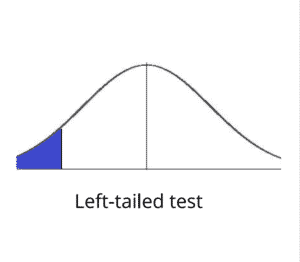
Reject H0: The common assumption in our example was that there is no difference in wing length of even the newly picked housefly. At the end of experiment, the wing length came out to be really small and is in the left most region of the housefly’s wing length data distribution shown in fig 1. As the outcome is in the left most extreme part of the distribution; hence, is at far most distance from the mean (wing length) of distribution.
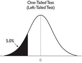
This is elaborated by diagram below. Our outcome is in the blue region of the distribution diagram below (fig 12).
Note: Ignore the meaning of “left tailed” test in fig 12 for now. This will become clearer as we go ahead in article.

fig 12: left tailed test based on housefly’s wing length

fig 13: possible outcomes of a left tailed test

This makes us think that there is a possibility that the disease is indeed widespread and is badly affecting wing length. This is because our sample outcome (In Blue region of fig 12) is not following the outcome that’s shown by most of the data in the current dataset (most data is in central region of the distribution shown in fig 12). Based on this idea, we reject the assumption about wing length made in the beginning of test that “The newly picked housefly’s wing length is no different from other housefly’s wing length.”

Fail to Reject H0: Now, suppose that the wing length came out to be in the center (or right most part) of the normally distributed data shown in fig 1 and fig 12.This makes us think that there is a high chance that there is no disease that’s prevalent in recent times that could affect wing length of houseflies. We can also say that the assumption -“The newly picked housefly’s wing length is no different from other housefly’s wing length.”- might be correct. We are still not sure that the assumption is correct because this is just an experiment done on one or few samples with the limited knowledge of pre-conditions. For example: we still don’t know about gender of houseflies or climatic condition that might affect the outcome of experiment. Hence, based on these arguments, we can say that we fail to reject the null hypothesis (assumption) rather than saying that we accept the null hypothesis.

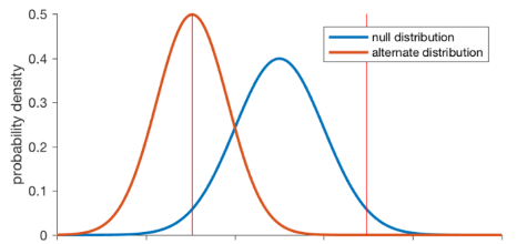
H0 and H1 distribution

An important thing to note is that during our entire discussion of hypothesis testing, we said that we reject Null Hypothesis if the outcome of experiment is in the left most extreme of the normally distributed data shown in fig 1. We can also say that in generic terms “if chances of the sample test outcome happening in real life, based on the given population distribution, is really low that it can be called as rarest of rare event, we can reject Null hypothesis”. In other words, it is highly likely that the sample outcome data belongs to a different distribution of data (Red colored distribution in fig 14) and not the one that we believed it to be (Blue colored distribution in fig 14) at the beginning of the test in fig 1 and fig 12. This is also shown in below picture.

fig 14: H0 distribution and H1 distribution

Now, an important point to note is that we did not discuss how extreme the experiment output should be for us to reject the null hypothesis. This is the next topic of discussion.

Level of significance

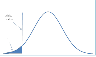
Let’s see a diagram first and then try understanding this concept.

As we know from density curve shown in fig 5 and distribution in fig 1, most of the population data resides in center of curve and few of the data resides in the corners. That means that there are very less houseflies with very high or very low wing lengths. These are rare occurrences. Now, for experiment, scientist wanted to prove that there is a disease affecting wing length and causing length to reduce a lot. For this to be proven, our observed data outcome needs to reside on the left most side of the curve (refer fig 15).

How do we define how much left of the curve’s mean our observed outcome need to be in order to be called a rare event so that we can reject H0? The answer is level of significance: alpha. Scientists working in medical domain have come up with a level of significance of 0.05 ~ 5% that’s broadly used in almost all the computations.

Let’s understand what it means to have 5% level of significance?

A 5% level of significance for a left sided test means that if our population data follows a standard normal distribution, only 5% of the entire data resides on the left side or in the black region of fig 16. The value on x-axis that marks the boundary for level of significance is called as critical point as shown in fig 15. Also, we can say that the area of curve in black region in fig 16 is 0.05. This is because total area under a relative density curve is 1 as proven before in the text shown between fig 2 and fig 3.

Now, lets try finding the critical point (x axis value or z score value) for our housefly wing’s dataset to clear the concept.

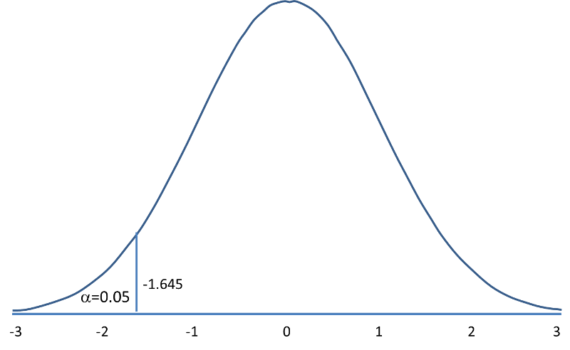
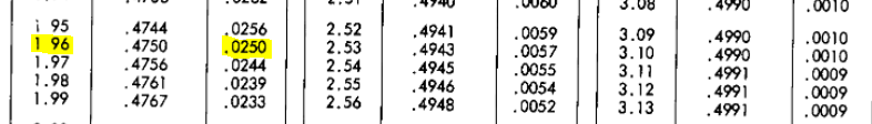
Based on the z-score table, we can see that to get “area beyond Z” value of 5%, we have an entry of .0505 ~ 5.05% in the table under section C as shown in fig 17. The z-score for this C value from the table is 1.64. This means that critical point on x axis is 1.64. This means that for a dataset represented by a standard normal distribution (refer fig 2 and fig 5), 5% of the entire population’s data resides on the left side of the curve (refer fig 16) i.e. 1.64 SD (z value of 1.64) from the mean zero of the curve. Since, it is a left sided test, the z-value of critical point will be negative i.e. -1.64 SD

fig 17: Z score table entries for housefly wing length dataset

fig 18: Critical (-1.645) value for left sided test. Level of significance is alpha (0.05 ~ 5%)

P-value

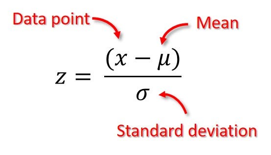
We discussed about an experiment being done by scientists earlier in this article to measure the wing length of a newly picked housefly to validate if there is a widespread disease limiting the length of wing. At the end of experiment, the wing length came out to be really small and in the left most region of the housefly’s wing length data distribution shown in fig 1. The wing length came out to be, lets assume, 38.99 mm. Now, we know the formula of converting a normal distribution into a standard normal distribution as shown below in fig 19. We know the mean and standard deviation of housefly dataset. Hence, we can compute Z-score for 38.99 mm value.

fig 19: Z score formula for converting a normal distribution to standard normal distribution.

fig 20: Mean and SD of wing length dataset

Z-score for 38.99 mm value = Standardized value for 38.99 mm = (38.99–45.5)/3.919647 = -1.661.

Since the critical value is -1.645 as shown in fig 18 and as per computation done above fig 18, our test outcome, -1.661, is to the left side of critical value.

Since test outcome z score < critical value; hence, we reject null hypothesis H0.

With this, we can also compute P-value which is nothing but the area to the left of our test outcome (-1.661) plotted on the distribution.

We compute this using Z score fig 21 as shown below. Area to the left of test outcome is same as area beyond z (C in fig 21) which is 0.0485 ~ 4.85%. This means there are only 4.85% of population data to the left of test outcome. We can say that there are 4.85% of house flies with wing length less than the wing length of house fly used for our test. This can also be seen visually in fig 22.

fig 21: p-value computation for test outcome

fig 22: p-value and z-score of test outcome

With the knowledge of above concepts, we can say that the curve shown in fig 18 can be divided into 2 areas as shown below in fig 23.

Rejection and Fail to Reject Regions

fig 23: rejection and non-rejection regions

Rejection Region: This is the area to the left of critical point in a left handed test.
Fail to Reject Region: This is the area to the right of critical point in a left handed test. We also see it called as acceptance region which sounds incorrect because we are not accepting H0 at all. We either reject H0 or fail to reject H0.

Next concept that we need to understand is the types of error in test.

Type 1 and Type 2 Errors

First, lets look at a diagram to visualize these errors alpha (type 1 error) and beta (type 2 error)

Type 1 Error — Alpha

When our test outcome falls in the “rejection region” but ideally it should have gone into the “Fail to reject region”, it is called as a False positive or Type 1 error.
We can also say that when we reject H0 but ideally we should have failed to reject H0, it is called as a False positive or type 1 error.
Based on our example, we can say that, the test outcome of wing length 38.99 mm (z-score 1.661) suggested us that there is indeed a disease causing wing length of housefly to remain less than usual, But, this outcome (widespread disease) was incorrect because our test subject was just an exception and there is no widespread disease affecting the wing length of housefly. This scenario is a false positive case or a type 1 error.

The probability of getting a type 1 error is same as level of significance (alpha) which is 5% in most of the cases. This level of significance is selected by scientist while conducting the experiment. If scientist would have selected a lower value for alpha, lets say 4%, we wouldn’t have Rejected H0 (our test outcome would fall in the “fail to reject region”) and hence, wouldn’t have got a False positive error.

Can we change level of significance — alpha value of 5%?

Yes, we can change the level of significance value. This truly depends on the dataset we are dealing with. If scientist is dealing with a crucial case, he can keep the alpha value to be 0.01 or even lower to avoid occurrences that occur by chance.
For example, Let’s say, we have a dataset containing blood test results of patients. Now, if z-score of conducted experiment (based on given blood test data) is less than critical value, we conduct a surgery else not. In this kind of a scenario, alpha is considered to be quite lower than 0.05.

Type 2 Error — Beta

When our test outcome falls in the “Fail to reject region” but ideally it should have gone into the “rejection region”, it is called as a False negative or Type 2 error.
We can also say that when we fail to reject H0 but ideally we should have rejected H0, it is called as a False negative or type 2 error.
Based on our example, we can say that, the test outcome of wing length 40.55 mm (z-score -1.263 : calculation done below this paragraph) suggested us that there is no disease causing wing length of housefly to remain less than usual, But, this outcome (No disease) was incorrect and there is indeed a widespread disease affecting the wing length of housefly. This scenario is a false negative case or a type 2 error.

Z-score for 40.55 mm value = Standardized value for 40.55 mm = (40.55–45.5)/3.919647 = -1.263

Another fun way to understand these errors is below picture from net.

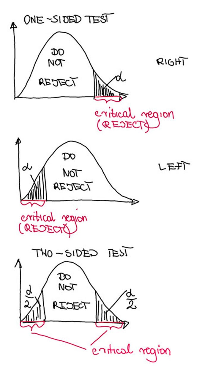
We kept mentioning about left sided test through out our article. There are other kinds of tests as well as explained below.

One sided Vs Two sided P-valued tests.

Whether we are doing a one sided test or a two sided test depends on the hypothesis test which is getting conducted. I have given some simple examples below to explain the concept.

If scientists want to test whether there is a virus that causes humans to become zombies, this is a left sided P-value test.
If scientists want to test whether there is a virus that causes extreme changes in humans (either makes them zombies or super humans), this is a 2 sided P-value test.
If scientists want to test whether there is a virus that causes humans to become superhumans, it is a right sided P-value test.

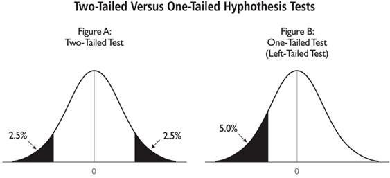
Two sided P-value test

An important difference that you might have noticed in a two sided P-value test is that the value of alpha: level of significance gets distributed into both directions as half and half as shown in fig 26 and fig 27. Hence, level of significance of 0.05 in a one sided test becomes 0.025 (alpha/2 ~ 0.05/2) on both sides of 2 sided p-value test. The critical value also changes in 2 sided p-value test because now, we need to look out for 2.5% of the area and not 5% of area in the Z score table. Please see fig 27 and fig 28 for visual explanation.