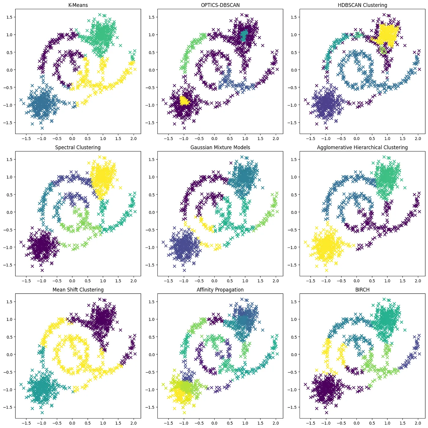
Comparing The-State-of-The-Art Clustering Algorithms
Let’s generate complex data and try different clustering algorithms
Here is the quick output: (Spoiler: My favorite one is HDBSCAN)
if you want to try yourself and play with parameters, here is the code:
import numpy as np
from sklearn.datasets import make_circles, make_blobs, make_moons
from sklearn.cluster import KMeans, OPTICS, SpectralClustering, AgglomerativeClustering, DBSCAN, MeanShift, AffinityPropagation, Birch
from sklearn.mixture import GaussianMixture
import hdbscan

# Generate the different structures
X1, y1 = make_circles(n_samples=200, factor=.5, noise=.05)
X2, y2 = make_blobs(n_samples=300, centers=[(1,1)], cluster_std=0.2)
X3, y3 = make_moons(n_samples=200, noise=0.05)
X4, y4 = make_blobs(n_samples=300, centers=[(-1,-1)], cluster_std=0.2)

# Combine all structures into a single dataset
X = np.vstack((X1, X2, X3, X4))
y = np.concatenate((y1, y2, y3, y4))

# Apply all the clustering algorithms
clustering_kmeans = KMeans(n_clusters=4, random_state=42).fit_predict(X)
clustering_optics = OPTICS(min_samples=10, xi=.01, min_cluster_size=.05).fit_predict(X)
clustering_hdbscan = hdbscan.HDBSCAN(min_cluster_size=10, gen_min_span_tree=True).fit_predict(X)
clustering_spectral = SpectralClustering(n_clusters=6, assign_labels='discretize', random_state=42).fit_predict(X)
clustering_gmm = GaussianMixture(n_components=6, random_state=42).fit_predict(X)
clustering_agglo = AgglomerativeClustering(n_clusters=4).fit_predict(X)
clustering_meanshift = MeanShift().fit_predict(X)
clustering_affinity = AffinityPropagation().fit_predict(X)
clustering_birch = Birch(n_clusters=6).fit_predict(X)
A quick look at the algorithms’ attributes:

Continue if you like to explore the algorithms one by one:
Let’s first start with a more complex dataset. We’ll create a dataset composed of five different shapes: two circles, two moons and a blob, each with different densities and added noise. This will serve as a challenging task for our clustering algorithms.
from sklearn.datasets import make_moons

# Generate additional structures
X3, y3 = make_moons(n_samples=200, noise=0.05)
X3 = X3 / 2 - 0.3  # scale and shift
y3 = 2*np.ones_like(y3)  # label for the new structure

X4, y4 = make_moons(n_samples=200, noise=0.05)
X4 = X4 / 2 + 0.3  # scale and shift
y4 = 3*np.ones_like(y4)  # label for the new structure

X5, y5 = make_blobs(n_samples=300, centers=[(-1,-1)], cluster_std=0.2)
y5 = 4*np.ones_like(y5)  # label for the new structure

# Combine all structures into a single dataset
X_large = np.vstack((X, X3, X4, X5))
y_large = np.concatenate((y, y3, y4, y5))

# Visualize the dataset
plt.figure(figsize=(8, 6))
plt.scatter(X_large[:, 0], X_large[:, 1], c=y_large, s=50, cmap='viridis')
plt.title('Original Dataset')
plt.show()
Here is the generated dataset. As you can see, it’s composed of five different structures: two circles, two moons, and a blob, each with a different density. This forms a challenging scenario for clustering algorithms and will help us evaluate their performance more effectively.
Now let’s move to the first clustering algorithm: K-means.
K-Means
K-means is a simple yet powerful clustering algorithm that assigns each data point to the nearest of a set of “centroids”, which represent the centers of the clusters. The centroids are iteratively updated to minimize the total within-cluster variance. However, K-means assumes that clusters are convex and isotropic, which is not always the case, especially with complex data.
Let’s apply K-means to our dataset and visualize the results.
from sklearn.cluster import KMeans

# Apply the KMeans algorithm
clustering_kmeans = KMeans(n_clusters=5, random_state=42)

# Fit the data
clustering_kmeans.fit(X_large)

# Visualize the results
plt.figure(figsize=(8, 6))
plt.scatter(X_large[:, 0], X_large[:, 1], c=clustering_kmeans.labels_, s=50, cmap='viridis')
plt.title('Clusters identified by K-Means')
plt.show()
As you can see in the plot above, K-means has some difficulties handling complex data shapes and varying densities. K-means is more suited to data with spherical clusters of similar sizes and densities.
Next, we’ll move to the OPTICS-DBSCAN algorithm.
OPTICS-DBSCAN
OPTICS (Ordering Points To Identify the Clustering Structure) is an algorithm that shares similarities with DBSCAN. It overcomes some limitations of DBSCAN by finding a basis of clustering structure from a set of density-based clusters. This is an advanced version of DBSCAN that uses a reachability distance concept to find the density-connected points.
from sklearn.cluster import OPTICS

# Apply the OPTICS DBSCAN algorithm
clustering_optics = OPTICS(min_samples=50, xi=.01, min_cluster_size=.05)

# Fit the data
clustering_optics.fit(X_large)

# Visualize the results
plt.figure(figsize=(8, 6))
plt.scatter(X_large[:, 0], X_large[:, 1], c=clustering_optics.labels_, s=50, cmap='viridis',marker = 'x')
plt.title('Clusters identified by OPTICS-DBSCAN')
plt.show()
As you can see in the plot above, OPTICS-DBSCAN has performed better than K-means on this complex dataset. It was able to identify clusters of different shapes and densities, although some areas of high density could be marked as noise.
HDBSCAN Clustering
Another popular density-based clustering algorithm is HDBSCAN (Hierarchical DBSCAN). HDBSCAN has an advantage over DBSCAN and OPTICS-DBSCAN in that it doesn’t require the user to choose a distance threshold for clustering, and instead only requires the user to specify the minimum number of samples in a cluster. This can make it more flexible and easier to use than DBSCAN or OPTICS-DBSCAN.
from sklearn.cluster import OPTICS

# Apply the OPTICS DBSCAN algorithm
clustering_optics = OPTICS(min_samples=50, xi=.01, min_cluster_size=.05)

# Fit the data
clustering_optics.fit(X_large)

# Visualize the results
plt.figure(figsize=(8, 6))
plt.scatter(X_large[:, 0], X_large[:, 1], c=clustering_optics.labels_, s=50, cmap='viridis',marker = 'x')
plt.title('Clusters identified by OPTICS-DBSCAN')
plt.show()
Spectral Clustering
Spectral Clustering is a technique that uses the eigenvectors of a similarity matrix to reduce the dimensionality of the data before performing another clustering algorithm (like K-means) in the reduced space. Spectral Clustering can identify complex structures and is especially good with non-convex clusters.
from sklearn.cluster import SpectralClustering

# Apply the Spectral Clustering algorithm
clustering_spectral = SpectralClustering(n_clusters=5, assign_labels='discretize', random_state=42)

# Fit the data
clustering_spectral.fit(X_large)

# Visualize the results
plt.figure(figsize=(8, 6))
plt.scatter(X_large[:, 0], X_large[:, 1], c=clustering_spectral.labels_, s=50, cmap='viridis')
plt.title('Clusters identified by Spectral Clustering')
plt.show()
As you can see in the plot above, Spectral Clustering was able to effectively identify clusters of different shapes and densities. It’s noteworthy that Spectral Clustering, unlike K-means and OPTICS-DBSCAN, has no concept of noise or outliers, so all points are assigned to a cluster.
Gaussian Mixture Models (GMM)
A Gaussian Mixture Model represents a composite distribution whereby points are drawn from one of several Gaussian distributions, each characterized by their mean and covariance. The expectation-maximization algorithm is used for learning the GMM parameters. GMM is a probabilistic model that assumes all the data points are generated from a mixture of a finite number of Gaussian distributions with unknown parameters.
from sklearn.mixture import GaussianMixture

# Apply the Gaussian Mixture Model algorithm
clustering_gmm = GaussianMixture(n_components=5, random_state=42)

# Fit the data and predict the labels
labels_gmm = clustering_gmm.fit_predict(X_large)

# Visualize the results
plt.figure(figsize=(8, 6))
plt.scatter(X_large[:, 0], X_large[:, 1], c=labels_gmm, s=50, cmap='viridis')
plt.title('Clusters identified by Gaussian Mixture Models')
plt.show()
As you can see in the plot above, Gaussian Mixture Models (GMM) have performed impressively on our complex dataset. GMM was able to identify clusters of different shapes and densities. This is because GMM, unlike K-means, can model elliptical clusters, and it provides soft clustering, meaning that each point belongs to each cluster to a different degree.
However, GMM can be sensitive to initialization values, can converge to a local optimum, and might not perform well when the clusters have different sizes.
Agglomerative Hierarchical Clustering
Hierarchical clustering algorithms build nested clusters by merging or splitting them successively. Agglomerative clustering is a type of hierarchical clustering that treats each data point as a single cluster and then successively merges the clusters that are closest to each other until only one cluster (or k clusters) remains.

As shown in the plot above, Agglomerative Hierarchical Clustering was able to identify the clusters quite effectively. This method builds a hierarchy of clusters, which is an added advantage as it provides more flexibility when you don’t know the exact number of clusters. However, it can be computationally expensive for large datasets.
Mean Shift Clustering
Mean Shift Clustering is a sliding-window-based algorithm that aims to discover “blobs” in a smooth density of samples. It is a centroid-based algorithm, which works by updating candidates for centroids to be the mean of the points within a given region. These candidates are then filtered in a post-processing stage to eliminate near-duplicates to form the final set of centroids.
from sklearn.cluster import MeanShift, estimate_bandwidth

# The following bandwidth can be automatically detected using
bandwidth = estimate_bandwidth(X_large, quantile=0.2, n_samples=500)

# Apply the Mean Shift algorithm
clustering_mean_shift = MeanShift(bandwidth=bandwidth, bin_seeding=True)

# Fit the data and predict the labels
labels_mean_shift = clustering_mean_shift.fit_predict(X_large)

# Visualize the results
plt.figure(figsize=(8, 6))
plt.scatter(X_large[:, 0], X_large[:, 1], c=labels_mean_shift, s=50, cmap='viridis')
plt.title('Clusters identified by Mean Shift Clustering')
plt.show()
As shown in the plot above, Mean Shift Clustering was able to detect and adapt to the complex structure and varying densities of our dataset. This algorithm doesn’t require the user to specify the number of clusters, as it determines the number of clusters based on the data. However, it requires a good choice of bandwidth, which can be difficult to find.
Affinity Propagation
Affinity Propagation is an algorithm that identifies exemplars among data points. Data points are seen as a network of peers. The algorithm exchanges real-valued messages between data points until a high-quality set of exemplars and corresponding clusters gradually emerges.
from sklearn.cluster import AffinityPropagation

# Apply the Affinity Propagation algorithm
clustering_affinity = AffinityPropagation(random_state=42)

# Fit the data and predict the labels
labels_affinity = clustering_affinity.fit_predict(X_large)

# Visualize the results
plt.figure(figsize=(8, 6))
plt.scatter(X_large[:, 0], X_large[:, 1], c=labels_affinity, s=50, cmap='viridis', marker='x')
plt.title('Clusters identified by Affinity Propagation')
plt.show()
As you can see in the plot above, Affinity Propagation did not converge on this dataset, meaning it could not identify a set of exemplars that were stable over successive iterations. This is one of the limitations of Affinity Propagation: it may not converge for some datasets or initial conditions.
Affinity Propagation also tends to create a large number of clusters compared to other methods, which can be a drawback depending on the application. It also has a higher time complexity, making it less suited for large datasets.
BIRCH (Balanced Iterative Reducing and Clustering using Hierarchies)
BIRCH is an algorithm designed to handle large datasets by first generating a more compact summary that retains as much distribution information as possible, and then clustering this summary. It is especially suited to large datasets, and can also incrementally process incoming instances.

As shown in the plot above, BIRCH (Balanced Iterative Reducing and Clustering using Hierarchies) was able to effectively identify clusters of different shapes and densities in our complex dataset. BIRCH is particularly well-suited for large datasets, and it has the advantage of being able to incrementally process incoming instances.
However, BIRCH only handles numeric data, and it may not perform well on high-dimensional data due to the curse of dimensionality.
Conclusion
We explored a variety of clustering algorithms, each having their own strengths and weaknesses. These include K-Means, OPTICS-DBSCAN, HDBSCAN, Spectral Clustering, Gaussian Mixture Models (GMM), Agglomerative Hierarchical Clustering, Mean Shift Clustering, Affinity Propagation, and BIRCH. My favorite one is HDBSCAN.
Algorithms like K-Means and GMM assume specific data distributions and thus may not perform well with complex datasets. Other algorithms, such as OPTICS-DBSCAN and HDBSCAN, do not require a predefined number of clusters, making them useful for datasets where the number of clusters is unknown. Hierarchical methods like Agglomerative Clustering and BIRCH provide a hierarchy of clusters, which can be useful for understanding the data at different levels of granularity.
However, no algorithm is universally superior, and the best choice often depends on the specific dataset and problem at hand. Factors such as the size and dimensionality of the data, the number of clusters, the shape and scale of the clusters, and the computational efficiency of the algorithm should all be considered when choosing a clustering algorithm.
Finally, it’s important to remember that clustering is exploratory in nature. The results should be used as a starting point for further analysis, and the assumptions and limitations of the chosen algorithm should always be kept in mind.
Thanks for reading!
You can follow me on Medium or LinkedIn and stay tuned for more articles on Data Science, Machine Learning, and AI.
If you are interested in learning more about my projects, check out my IBM skills network profile: