Stock Market Prediction- An Automated Approach

It has been a few days when suddenly I was asked as to predict to buy or sell stocks of a company on the basis of its given data. So, when should one buy the stocks, when should one sell them?

Most of the ML models predict the closing prices using different Machine Learning algorithms and give the f1 score and roc details to their model. However, the accuracy is generally not very high. In my view, this is because we just primarily focus on the closing prices and not the other factors of the data.

In this article, I would discuss an LSTM sequential model that is used to predict closing prices and opening prices of a company.

Dataset : Amazon’s stock data taken from yahoofinance site. Go to link: https://in.finance.yahoo.com/quote/AMZN/history?p=AMZN.
Change the time period to MAX and then click on apply. After the data gets loaded. Click on download to save it in your PC. It would be saved as ‘AMZN.csv’.

I have used Google Colaboratory for the entire python coding. Now I will start showing you the steps. First of all, Import the required libraries.

import pandas as pd
import numpy as np
import keras
import tensorflow as tf
from keras.preprocessing.sequence import TimeseriesGenerator as tg

Call the data.

from google.colab import files
uploaded = files.upload()

Google Colab will ask you to upload the file. Select “choose file” to upload the ‘AMZN.csv’ file.

Now convert the file to pandas dataframe. Then preview the first 5 rows data.

data = “AMZN.csv”
df = pd.read_csv(data)
df.head()

Amazon data first 5 rows since May 1997

Analyse the data

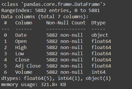
df.info()

No of rows and columns

Now, the date needs to be converted as a relevant data, i.e. We will tell pandas that the data in the column named “Date” needs to be read in the date-time format. This is exactly like telling the computer to read 5 as integer and “Apple” as a string.

df[‘Date’] = pd.to_datetime(df[‘Date’])
df.set_axis(df[‘Date’], inplace=True)
df.drop(columns=[‘High’, ‘Low’, ‘Volume’], inplace=True)

We will keep the Open and Close data in the dataframe and drop the high, low and volume data as we are not using this in the prediction.

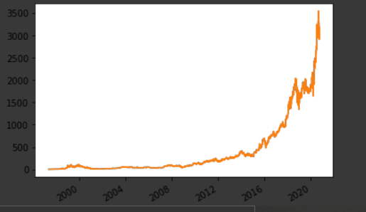
Now let us visualize the Open and the close data.

df[“Close”].plot()
df[“Open”].plot()

The Y axis defines stock prices and the X axis define the years

In the graph, there are two curves of orange and blue color. Both of them almost seem to overlap. This is because on a particular date, Open and close prices do not have much difference in their values.

Now we will define the different datasets that we would require to create the testing and training data.

open = df[‘Open’].values
open = open_data.reshape((-1,1))
close = df[“Close”].values
close = close_data.reshape((-1,1))
k = 0.6 # The ratio of data you want to keep as training to the total data
split = int(k*len(open))
open_train = open_data[:split]
open_test = open[split:]
close_train = close[:split]
close_test = close[split:]
date_train = df[‘Date’][:split]
date_test = df[‘Date’][split:]

Now create the testing and training data and we will take the length of the data to be 30 days.

train_generator = tg(open_train, close_train, length=30, batch_size=40)
test_generator = tg(open_test, close_test, length=30, batch_size=1)

Create the LSTM Sequential Model. The first layer is activated using tanh function and the input layer is (30,1). The model is fitted and iterated a hundred times.

from keras.models import Sequential
from keras.layers import LSTM, Dense
model = Sequential()
model.add(LSTM(64,activation=’relu’,input_shape=(30,1)))
model.add(Dense(1))
model.compile(optimizer=’adam’, loss=’mse’)

model.fit_generator(train_generator, epochs= 100, verbose=2)

After running this cell, the 100 epochs will run and the losses would be shown.

Now visualizing the data. Comparing the model predictions of testing data set and the actual values.For this we will have to import graph objects to the code. Then we will plot the stocks to understand the variations.

import plotly.graph_objects as go
prediction = model.predict(test_generator)
open_train = open_train.reshape((-1))
open_test = open_test.reshape((-1))
close_train = close_train.reshape((-1))
close_test = close_test.reshape((-1))
prediction = prediction.reshape((-1))
training_graph = go.Scatter(x = date_train,y = close_train,mode = ‘lines’,name = ‘Data’)
Test_prediction_graph = go.Scatter(x = date_test,y = prediction,mode = ‘lines’,name = ‘Prediction’)
testing_graph = go.Scatter(x = date_test,y = close_test,mode=’lines’,name = ‘Original Data’)
layout = go.Layout(title = “Amazon Close_Prices”,xaxis = {‘title’ : "Date"},yaxis = {‘title’ : “Close from Open”})
fig = go.Figure(data=[training_graph, Test_Prediction_graph, testing_graph], layout=layout)
fig.show()

We can see the difference in predicted price and the actual price.

Now let us check the accuracy of the model. Since trade markets are very vulnerable a stock price cannot be predicted exactly to a value as the original one. There is no set pattern on which the data changes. So we would keep a sensitivity of 2% of the average close price of 2020. From the graph, in 2020, the stock prices have risen from 2200 to 4000 approximately.

2% of 3100 = 62.

d =0
for i in range(len(close_test)):
 for j in range(len(prediction)):
  if i == j:
   if (close_test[i] — prediction[j])<62:
    if (close_test[i] — prediction[j])>-62:
     d = d+1
print(d/len(close_test))

On running this cell, the accuracy comes out to be 65.1%

Now we will forecast the data

close_data =close_data.reshape((-1))
def predict(n, model):
 prediction_list = close_data[-look_back:]
 for _ in range(n):
  x = prediction_list[-30:]
  x = x.reshape((1, 30, 1))
  out = model.predict(x)[0][0]
  prediction_list = np.append(prediction_list, out)
 prediction_list = prediction_list[29:]
 return prediction_list
def predict_dates(num_prediction):
 last_date = df[‘Date’].values[-1]
 prediction_dates = pd.date_range(last_date,periods=num_prediction+1).tolist()
 return prediction_dates
forecast = predict(10, model)
forecast_dates = predict_dates(10)
print(forecast_dates)

[Timestamp(‘2020–09–28 00:00:00’, freq=’D’), Timestamp(‘2020–09–29 00:00:00’, freq=’D’), Timestamp(‘2020–09–30 00:00:00’, freq=’D’), Timestamp(‘2020–10–01 00:00:00’, freq=’D’), Timestamp(‘2020–10–02 00:00:00’, freq=’D’), Timestamp(‘2020–10–03 00:00:00’, freq=’D’), Timestamp(‘2020–10–04 00:00:00’, freq=’D’), Timestamp(‘2020–10–05 00:00:00’, freq=’D’), Timestamp(‘2020–10–06 00:00:00’, freq=’D’), Timestamp(‘2020–10–07 00:00:00’, freq=’D’), Timestamp(‘2020–10–08 00:00:00’, freq=’D’)]

These dates for which the stock prices would be predicted are printed.

Now print the forecast values.

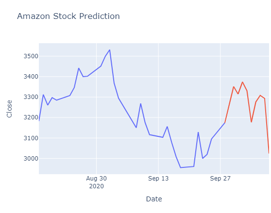
[3174.050049 3263.98950195 3351.03442383 3314.97192383 3373.79077148 3331.03149414 3176.78857422 3275.86425781 3307.94433594 3293.53564453 3023.87182617]

t1 = go.Scatter(x = date_test[-30:],y = close_test[-30:],mode=’lines’)
t2 = go.Scatter(x = forecast_dates,y = forecast,mode=’lines’)
layout = go.Layout(title = “Amazon Stock Prediction”,xaxis = {‘title’ : “Date”},yaxis = {‘title’ : “Close”})
fig = go.Figure(data=[t1, t2], layout=layout)
fig.show()

Close price on 28th September, 2020: 3174.09

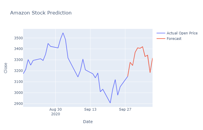
Similarly, by replacing the close_test data in forecast function, you should predict the open prices also.

Open Price on 29th September: 3277.579

Now we will check the Open Price on 29th September, 2020 and compare it with 28th September, 2020 Close Price. NOTE: These dates are for my data that I have downloaded. In your case, you will compare Open Price’s red graph’s second date with Close Price’s red and blue graph intersecting date.

If Open Price tomorrow is greater than today’s Close Price, we should buy the stocks and vice versa. You could create a code for this as well.

if forecast_close[0]<forecast_o[1]:
 print(“Buy the Stocks”)
else:
 print(“Sell the Stocks”)

So actually, from the model, we predict that we should buy the stocks on 28th September, 2020. Let us compare it with the actual 28th September, 2020 and 29th September, 2020 data.

So from this data also, we conclude that we should buy the stocks as the price has increased.

Surely from here the predicted opening price has an approximate difference of 50 units, which is approximately 1.7% in difference.

So if you want to become a trade in stocks, you could use this model, or you could even improve this model.

You could also change the activation from tanh to relu, decrease the neural network layers from 64 to a lower value. However, this might increase overfitting of data.

One could also create a simple sequential model to check if we have to buy or sell the stocks using binary classifiers.

I am open to suggestions.

Thanks!