Scaling ClickHouse: Achieve Faster Queries using Distributed Tables
Introduction
ClickHouse is an open-source Online Analytical Processing (OLAP) database system. It is renowned for its blazing speed, horizontal scaling, and ability to serve big data for time-series and other types of analytics. ClickHouse can scale horizontally by adding more nodes to the cluster. This approach distributes data and compute jobs across multiple nodes, enhancing overall performance.

If you are not familiar with ClickHouse, or looking for a beginners’ guide, I recommend reading my previous article that covers the basics of ClickHouse, goes through its core concepts, and provides hands-on demonstration of its capabilities.
This article covers using Distributed tables in ClickHouse to enhance filtering and aggregation performance.
Distributed Engine — and distributed tables
Distributed engine is used to create distributed tables. Table created with Distributed engine is a virtual entity, and doesn’t hold any data. It is created on top of actual tables, that can have one of many engines provided by ClickHouse’. The Distributed engine enables distributed queries on the underling actual tables, called shards.
The mechanism to create distributed tables is:
- Create tables on cluster nodes
- Create the distributed table on top of those tables created on each node
The underlying tables are standard tables that contain the actual data. Distributed table is a virtual entity on top that enables distributed queries and data insertions.
To read more about the Distributed engine, please refer to the following link:
Following is the syntax of creating distributed tables:
Alternatively, if one of the underlying tables exist on the same host that distributed table is being created on, it is possible to use that schema instead of defining it, by using the AS clause:
In the syntax, the following parameters are important:
table_name: The name of the distributed tablecluster: The cluster on which table is to be createddatabase: The name of the database to create the table insharding_key: It is an optional parameter. It is required when inserting data into the distributed table. When data is inserted into the distributed table, thissharding_keyparameter value is used to route each row to the correct underlying table. Alternatively, it is possible to add data into the underlying tables directly. The sharding key needs to be numeric. Because is an expression, it can be any expression containing table columns that returns an integer.
Inserting data into Distributed table and its population in shards
There are two ways to insert data into the distributed table:
- Insert data into the shards i.e. the underlying tables directly. This approach is the most flexible as it allows maintaining any sharding mechanism, and according to the documentation, it is also the most optimized, and allows complex sharding logic that can be implemented outside ClickHouse. This mechanism is also recommended for large volume of data.
- Inserting data directly into the distributed table, and letting it route the rows to appropriate shards. Using this mechanism requires specifying the
sharding_keyparameter on the Distributed table. Each row is inserted into the appropriate shard based on the sharding key.
The two mechanisms can be depicted as the following diagram:

Each shard can have a weight, and default weight is 1. The weight determines the proportion of the rows sent to that shard, when they are inserted into the distributed table instead of direct insertion to the replicas. The mechanism works by evaluating the shading expression of each new row, and taking a remainder by dividing that value by the total weight of the shard. The remainder then determines which shard the data is inserted into.
If there are 3 shards, two with weight 2, and third with weight 5, the total weight is 2 + 2 + 5 = 9. The remainder is computed by dividing the output of sharding expression of the row by 9. Then the data with remainders 0 and 1 (it is 0 inclusive to 2 non-inclusive) go to the first shard, the data with values 2 and 3 (values 2 inclusive to 4 non-inclusive) go to the second shard, and the data with remainders 4 to 9 go to the third shard.
If all shards have a weight of 1, then remainder 0 go to the first shard, 1 go to the second shard and so on. Also, in this case the data is equally distributed. When a new shard is added, by setting its weight higher, its “acceptance range” of remainders can be increased so that it can get filled up quicker.
Note that if the shards are replicated, then the data is written to all replicas simultaneously by the distributed table, if written to the distributed table directly. According to the documentation, this is not efficient and leads to inconsistencies among replicas of the shards. Therefore, it is recommended to set internal_replication parameter to true for shards that belong to the ReplicatedMergeTree family. When internal_replication is set to true, data is written to the first healthy shard. The data is then internally distributed to the remaining shards.
For more details, refer to the documentation: https://clickhouse.com/docs/en/engines/table-engines/special/distributed#distributed-writing-data
Querying data from distributed table
The main advantage of using Distributed table is to spread the data, to improve query performance. Filters and aggregations are processed by multiple nodes to produce the final results quickly. The select queries are sent to all shards.
Hands-on — Insertion and Querying data in distributed table
Now, lets go through an example of insertion of data into ClickHouse distributed table, and querying it. Additionally, we’ll compare query performance compared to a table that has only one shard and exists on only one node. For that, we need a ClickHouse cluster. Lets create one, a 3 node 1 replica cluster using Docker Compose:
Create a test ClickHouse cluster
The ClickHouse cluster created here consists of 3 Docker container nodes, each having 4GB RAM, and uses 2 CPU cores. The laptop I am using has Apple M1 processor and 16GB RAM. If you are running on a different machine, you can adjust accordingly. First, clone to the code repository that I have created container the Docker file and the docker-compose file:
Make sure you have Docker and Docker compose installed. I prefer using Docker Desktop locally, as it has a nice UI as well. If you do not have Docker installed, install it first by visiting the following link:
Next, with Docker running, open a terminal, and cd into the repository, and run docker compose up:
The cluster should start shortly:

Next, connect to the cluster. The URL of the nodes is:
Node 1: localhost:8123
Node 2: localhost:8124
Node 3: localhost:8125
You can connect with all 3 nodes using the default user and no password.
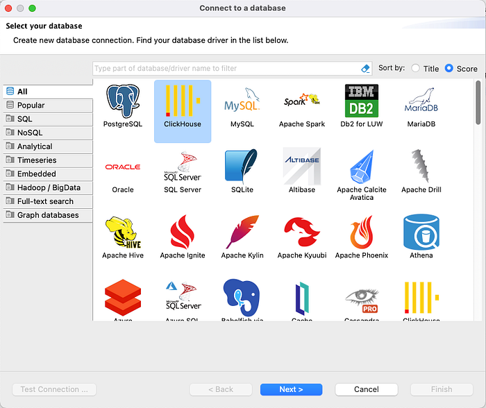
I prefer using DBeaver Community Edition. It can connect to ClickHouse, and also to older versions using ClickHouse legacy driver:

DBeaver may download the ClickHouse driver when creating connection for the first time.


n addition to that, ClickHouse client, which is a command line tool, can also be used. Link:
This set-up has been explained in more detail in my article:
Downloading example data — TLC Trip Records data
I like using TLC Trip Records data, which is a dataset of Taxi trips in New York city. It can be downloaded from:
For this demonstration, I am using Yellow Trip Record files for year 2023. Download the Yellow Taxi Trip Record Parquet files for all months of 2023:

In the ClickHouse repository, there is a folder called data. This folder has been mounted to all 3 nodes at path /var/lib/clickhouse/user_files. In the data folder, there is a folder rides_2023. You can place all the files there, and they become available to all ClickHouse nodes.
Loading data into ClickHouse — table on a single node
First, create a database, and a table to hold raw data using the following commands. Execute them on node 1:
rides database, and the trips_raw tableThe above commands that were just executed do the following:
- Creates a database called
rideson all 3 nodes. Note that any command executed with theON CLUSTERclause is executed on all nodes of the cluster. - Creates a table called
trips_rawon the node this command was run on, i.e. node 1.

The table uses the MergeTree engine, which is one of the table engines available in ClickHouse. You can refer to the documentation of MergeTree engine family, or my previous article to learn more about table engines available in ClickHouse.
Next, load the data into the table, this can be done using the following command:
This command needs to be executed on the instance itself, so, connect to node 1. Open a new terminal and run:

ClickHouse client is already installed on all nodes, and connects to the locally running ClickHouse node. Now, run the command to load the data:

We can run a count query on the table to verify that the data has been loaded:

Next, lets create a trips table, and load data into it. Run:
The commands to load data into the trips table have been split into 4 parts because, due to limited resources present in this test cluster, tying to load all the data at once results in out of memory errors. You can split the data further if these commands still give an error at your end, and use SELECT max(trip_id) FROM rides.trips t; to get the maximum trip_id value to put in the next insert query.
After loading the data, lets run a row count:

Note that the final number of rows is a little different compared to the raw data because there are some rows that have dates in years other than 2023, and they get filtered out.
Creating and loading data into the distributed table
Next, lets create a distributed table, called trips.rides_distributed_id. The trip identifier column, trip_id is the shading key in this table, and this case, it’ll be a numeric column as it is a requirement. Note that the sharding key is an expression, so if the column itself is not numeric, the sharding key expression can return a numeric result.
Also, as explained earlier, Distributed table in ClickHouse is a virtual entity over real tables on all nodes, and that the distributed table itself doesn’t hold any data. Therefore, a table called rides.trips_part_dist_by_id also needs to be created on all three nodes.
To do both, run the following commands:
Because the CREATE TABLE query contains the ON CLUSTER clause, the table rides.trips_part_dist_by_id gets created on all three nodes. Additionally, we use the ON CLUSTER clause in the code to create distribution table, it gets created on all nodes. If this clause is omitted while creating the distributed table, the distributed table gets created only on the node the command runs on.
Next, load data into the distributed table:
In the insert statements, the data gets inserted directly into the distributed table, and gets routed to the appropriate partition based on the trip_id column value.
After execution of the commands, the following tables are present on each node:

Query performance comparison
Let’s run a query that computes average tip distance, fare amount, and tip amount for each pickup location ID, and orders by highest average tip amount in descending order. The query is:
If the query is run on ClickHouse client, I get the following results on my system:

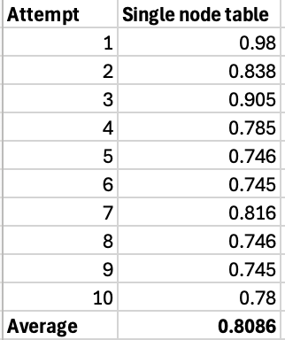
This query can be executed using a client such as DBeaver, but ClickHouse client provides more information, including a more precise execution time, and number of rows touched etc. On my computer, it took 0.98 seconds.
Lets run it for 10 times. The execution times are:

Most of the times the query took approximately 0.75 seconds, and average time is 0.8086 seconds overall. Next, lets run the same query on the distributed table:

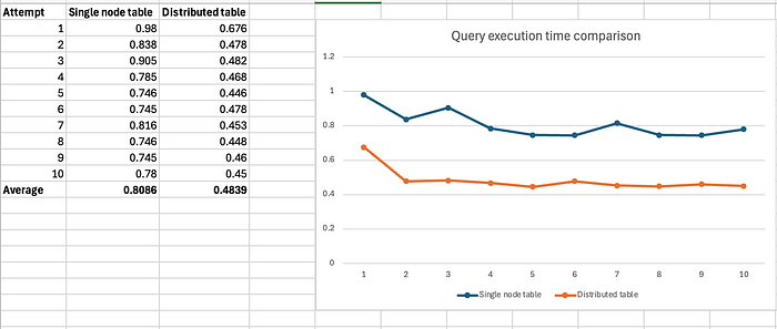
On the distributed table, the query took 0.676 seconds on the first attempt. Running it for 10 times. The average time taken by running the same query on the distributed table is 0.4839 seconds.
Here is the comparison:

The advantage of using a distributed table can be clearly seen here, as the data is distributed, the query is also distributed, and the results are generated faster. In this example, on my computer, the query on distributed table runs 40.16% faster.
This is a massive difference. In real world, there would be additional time taken by sending data over the network to combine the overall result, but the tables and possibly the ClickHouse cluster would be bigger as well, do the difference could be significant.
Lets compare the query plans of both queries:

The difference here is the ReadFromRemote step, which indicates that the parts of the query were executed on other nodes. Overall, this division of work leads to faster execution.
Note: A nice article and video about query plans in ClickHouse can be found here:
Next, lets examine another example, which involves a filter in addition to grouping and aggregates. The query is:
The execution time comparison is:

This query takes and average of 0.7527 seconds, whereas the same query on the distributed table takes 0.4713 seconds on average. The query on the distributed table is 37.39% faster. This again demonstrates that advantage of using distributed table.
Although distributed tables add complexity, they significantly improve query processing by spreading both data and execution across multiple nodes. This horizontal scaling approach is a valuable strategy for ClickHouse, enabling it to handle large datasets and process queries more efficiently. The performance gains achieved through this method make it a worthwhile investment for organizations dealing with substantial data volumes.
Conclusion and Key Takeaways
In conclusion, distributed tables in ClickHouse offer significant performance gains for large-scale data processing. By spreading data and query execution across multiple nodes, ClickHouse achieves faster query times by distributing the workload. Designed to handle massive datasets, ClickHouse offers tools like distributed tables to enhance query performance and improve scalability.
