Artificial Neural Network using R Studio
Assalamualaikum wr.wb.
Hi everyone!
Actually, this is my very first story in Medium. So without any further due, let’s we’re going onto the main topic.

An artificial neural network (ANN) is a computer simulation of the human brain in its most basic form. A normal brain can adapt to different and changing environments and learn new things. The brain has the incredible capacity to evaluate partial, ambiguous, and fuzzy information and generate its own conclusions (Kukreja et al., 2016).
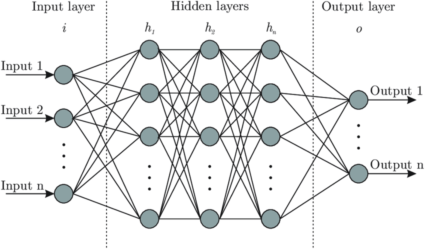
The ANN design consists of :
- an input layer that receives input values
- a hidden layer(s) that fits between the input and output levels and contains a group of neurons (which could be a single layer or several layers)
- an output layer that usually contains a neuron.
Its output is in the range of 0 to 1, or more than 0 and less than 1. However, several outputs are possible.
The dataset that used in this story is the Breast Cancer Wisconsin (Diagnostic) Data Set by Kaggle. Here’s the link: https://www.kaggle.com/uciml/breast-cancer-wisconsin-data. The dataset will be analyzed using ANN single layer and multilayer.
Let me explain the steps to analyze using ANN Method in R Studio by order.
- Inputting and checking the structure of data
Dataset <- read.csv(file.choose(), header = TRUE, sep = “,”)
Dataset
str(Dataset)
According to the figure of the dataset, we know that the only variable identified as a character is the first variable (diagnosis). Then we also know that the other variables are identified as numeric.
2. Checking missing data in the dataset using R Studio's “summary” function.
summary(Dataset)
Since the output of summary data doesn’t contain NA’s value, it means none of the missing data was there.
3. The “diagnosis” variable is defined as a dependent. However, it is a character, so we need to categorize and change it into numeric. Here’s the code that we should type in R Studio
library(dplyr)
Dataset[,1]=sapply(Dataset[,1],switch,”B”=0,”M”=1)
Dataset[,1] #0:benign(B), 1:maligant(M)
str(Dataset)
The “diagnosis” variable has changed onto numeric.
4. Then, the next step is determining which variables we will use. We will use every “worst” variable (or the 22nd till the last variable) and define it as a new dataset called “Dataset2”. Here’s the R code.
Dataset2 <- Dataset[c(1,22:31)]
Dataset2
5. Scaling the data using the min-max scaler.
for (i in names(Dataset2[,-1])) {
 Dataset2[i] <- (Dataset2[i] — min(Dataset2[i]))/(max(Dataset2[i]) — min(Dataset2[i]))
}
6. Partitioning the data into two, test and train with a 75:25 ratio.
set.seed(222)
newdata <- sample(2, nrow(Dataset2), replace = TRUE, prob = c(0.75, 0.25))
training1 <- Dataset2[newdata==1,]
testing1 <- Dataset2[newdata==2,]
The backpropagation algorithm is the most often used methodology for neural network training. The difference between the predicted and actual output is propagated back to the layers, and the weights are changed (Kukreja et al., 2016).
7. Artificial Neural Network Single Layer
Training data using the “neuralnet” package in R and defining the number of hidden layers of the created neural network. We use 3 hidden layers, with the Diagnosis variable as the dependent.
library(neuralnet)
set.seed(333)
n3 <- neuralnet(diagnosis~.,
 data = training1,
 hidden = 3,
 err.fct = “ce”,
 linear.output = FALSE)
plot(n3)
Here is the neural network plot obtained.

The figure above showed that the neural network has 10 inputs (radius, texture, perimeter, area, smoothness, compactness, concavity, concave points, symmetry, and fractal) and 3 neurons, which are the hidden layer lead to the weight value. The weight value is the inter-unit connection strength that is used to maintain processing capabilities. Last but not least, the blue number is also known as the bias.
The error value shows the loss of training data. Then, we got 0.065446 to lose our training data. The steps are the number of iterations by the machine, so we got 22280 total iterations.
Here is the R code to get the prediction model.
# Prediction #
output3 <- compute(n3, testing1[,-1])
head(output3$net.result)
head(training1[1,])results3 <- data.frame(DataAsli=testing1$diagnosis, Prediksi=output3$net.result)
results3library(caret)
roundedresults3 <- sapply(results3, round, digits=0)
roundedresults3
Here is the accuracy that we got using a confusion matrix
actual1 <- round(testing1$diagnosis, digits = 0)
prediction3 <- round(output3$net.result, digits = 0)
mtab3 <- table(actual1,prediction3)
mtab3
confusionMatrix(mtab3)
The figure shows that we got 76 data Benign (0) that classified as Benign (0), 3 data Benign (0) that classified as Malignant (1), 4 data Malignant (1) that classified as Benign (0), and 44 data Malignant (1) that classified as Malignant (1) while we are using ANN 3 layers. We also got 0.9449 as accuracy or equal to 94.49%, and another 5.51% defined as an error. The Kappa index has 0.8823, which the value has greater than 0.75, which means the ANN layers 3 that we used is excellent.
8. Artificial Neural Network Multilayer
In general, the steps to get ANN multilayer is the same way to get ANN single layer. The only difference between them is the value of “hidden” in the R code we used. Here is the R code of the ANN multilayer.
library(neuralnet)
set.seed(333)
n25 <- neuralnet(diagnosis~., data = training1, hidden = c(2,5),
                 err.fct = “ce”, linear.output = FALSE)
plot(n25)
We used 2 layers and 5 layers, so here is the neural network plot obtained.

The figure above showed that the neural network has 10 inputs (radius, texture, perimeter, area, smoothness, compactness, concavity, concave points, symmetry, and fractal), 2 neurons, and 5neurons, which are the hidden layer lead to the weight value. We got 11.898758 errors and 16324 total iterations.
Here is the R code to get the prediction model.
# Prediction #
output25 <- compute(n25, testing1[,-1])
head(output25$net.result)
head(training1[1,])results25 <- data.frame(DataAsli=testing1$diagnosis, Prediksi=output25$net.result)
results25library(caret)
roundedresults25 <- sapply(results25, round, digits=0)
roundedresults25
Here is the accuracy that we got using a confusion matrix
prediction25 <- round(output25$net.result, digits = 0)
mtab25 <- table(actual1,prediction25)
mtab25
confusionMatrix(mtab25)
The figure shows that we got 76 data Benign (0) that classified as Benign (0), 3 data Benign (0) that classified as Malignant (1), 3 data Malignant (1) that classified as Benign (0), and 45 data Malignant (1) that classified as Malignant (1) while we are using ANN 3 layers. We also got 0.9528 as accuracy or equal to 95.28%, and another 4.72% defined as an error. The Kappa index has 0.8995, which the value has greater than 0.75, which means the ANN multilayer 2,5 that we used is excellent.
Resume
We use the “neuralnet” package in R Studio for analyzing Artificial Neural Networks. The dependent variable in ANN should be numeric, so whenever you have a character one, you need to categorize it or turn it into numeric.
ANN multilayer 2,5 is better than ANN single layer 3 because ANN multilayer 2,5 has higher accuracy than ANN single layer 3.
Here we come to the end of the story. I would say thank you very much and also see you on another story!
Wassalamualaikum wr.wb.
Best regards,
Sukma Anindita.
References
Kukreja, H., N, B., S, S. C., & S, K. (2016). AN INTRODUCTION TO ARTIFICIAL NEURAL NETWORK. International Journal Of Advance Research And Innovative Ideas In Education, 1(5), 27–30. https://doi.org/10.2514/6.1994-294
Lek, S., & Park, Y. S. (2008). Artificial Neural Networks. Encyclopedia of Ecology, Five-Volume Set, 237–245. https://doi.org/10.1016/B978-008045405-4.00173-7
