Face Mask Detection algorithm using Convolutional Neural Network — AI — Computer Vision
In this article, we explore an application of Computer Vision that is largely relevant to the global health crisis that is the Coronavirus. As many countries continue their desperate fight to control the infection rate and spread of the virus, we have seen the integration of many unfamiliar; and somewhat inconvenient, protection measures being introduced into society over the past 6 months. One of these particular measures; at least in the UK, is the mandatory requirement of wearing a protective face mask in shops, cafes, restaurants, and other compact or enclosed social environments. This project looks at automating the task of checking whether someone is wearing a protective mask through the development, training, and deployment of a Computer Vision ML model. The specific Machine Learning model used in this project is the widely popular Convolutional Neural Network (CNN).
Starting with the end in mind, we will first take a look at the demonstration video which shows the trained CNN model in action. Here the model is attempting to classifying images from a live webcam feed into one of two target categories: “Wearing a mask”, or “Not wearing a mask”. This is the product that will be developed within this project.
Before diving deep into the logic and code that the project encompasses, it is good to provide an overview of what exactly a Convolutional Neural Network is and why it is one of the most popular Machine Learning algorithms for Computer Vision tasks. We will then take a comprehensive walkthrough of the project, discussing and understanding each step and how it contributes towards the end goal of a fully trained and optimized model that is ready for deployment. This walkthrough will contain 4 major subsections:
- Acquisition and exploration of the training/testing dataset
- Data pre-processing,
- CNN architecture development, training, and testing
- Model deployment for live webcam feeds
Project code can be found on my GitHub page: (Link)
What is a Convolutional Neural Network, and how does it work?
This supporting information has been taken and adapted by Sumit Saha’s article “A Comprehensive Guide to Convolutional Neural Networks — the ELI5 way” which can be accessed from the references section of this article.

The agenda for Computer Vision is to enable machines to view and perceive the physical world in similar ways to how us humans do. This includes the ability to accurately and reliably carry out a multitude of image-based tasks including, but not limited to:
- Analysing & Classifying objects (“is this a picture of a cat, or a dog?”)

- Object Recognition (“Can you recognize and label everything in this image for me”),

- Media Recreation (“What would the Mona Lisa look like if it was painted in the style of Vincent Van Gogh?”) — probably something like the middle re-creation below.

The advancements in computer processing power and complexity, and data capturing and storage, through time and continuous expert hardware engineering have helped AI enthusiasts overcome previous significant blockers that prevented earlier adoption of Computer Vision tools and techniques in everyday use. Now, in 2020, such Computer Vision applications are; and continue to be, implemented in many aspects of everyday life; from quirky filters and backgrounds on Snapchat images/videos to Smartphone security with Retina or Full Face scans to proximity detection in car sensor systems, to name but a few. The Convolutional Neural Network is what drives much of the decision-making behind these algorithms. But how exactly does it work?
Introduction — Convolutional Neural Network

A Convolutional Neural Network is an algorithm that can take in an image as input, assign importance (in the form of trainable weights and biases) to aspects or features of the image and output a decision or some other form of logic based on what it has “seen” in the image. The data pre-processing / preparation required is very minimal when it comes to CNN architectures as the features of your data are the actual pixel values and with enough training data, CNN will automatically define which of these pixels are most important in its decision-making. (Sumit Saha, 2018)
Why choose CNN over Feed-Forward NN?

Any image stored electronically is just a matrix of pixel values ranging from 0 (Black) to 255 (White), with values in-between this range indicating the “Greyness” of the pixel — the closer the value to 0, the darker the grey (and vice versa).
So why not just flatten this matrix into a single vector of pixels and feed it directly into a Multi-layer Perceptron Neural Network, where each pixel corresponds to an input neuron? It’s not quite as easy as that…
In the case of a standard feed-forward NN, each input neuron would directly map to a feature in the dataset, and the assumption here is that each neuron (and thus feature) is completely independent of each other. However, this is not the case for image data. Pixels in an image have both Spatial and Temporal dependencies — if you imagine an image of the moon in the night sky, you would expect all of the pixels near the moon to have similar pixel values (they should all be around 200–255), and the further away from the moon the pixel is, the darker the pixel becomes (and closer it’s value reduces towards 0). A standard feed-forward Neural Network would not be able to preserve this type of Spatial and Temporal information and it’s performance is constrained to the information it can gain from each individual pixel in the image without considering other pixels nearby.
The Convolutional Neural Network, on the other hand, can capture these dependencies through the application of relevant filters. The architecture performs a better fitting to the image dataset due to the reduction in the number of parameters involved and the reusability of weights. In other words, the network can be trained to understand the sophistication of the image better.
CNN Input Images

In the figure to the left, we have a RGB image which is separated into its three colour planes — Red, Green, and Blue. The dimensions of this very basic image are 4 x 4 x 3 — four pixels in height and width, and three colour channels.
The above 4 x 4 image has 16 pixels per colour channel. For an RGB image, this would equal a total of 16 x 3 (colour channels) = 48 pixels. You can imagine how computationally intensive this would become once our images reach much higher dimensions. For example, an 8K image with dimensions (7680 x 4320 x 3) would equal a total of 99,532,800 pixels per image! One of the major roles of the CNN is to reduce these images into a form which is easier to process, without losing the features that contribute heavily towards its predicting capability. This is paramount when we come to design an architecture that is not only good at deriving the features in the image but can also scale well to massive image datasets (think tens of thousands of images and above).
Convolutional Layer — The Kernal

Example image dimensions: 5 (height) x 5 (width) x 3 (colour channels) = 75 pixel total.
In our example image to the left, the green section represents our matrix of image pixels, and the smaller yellow matrix is the kernal/filter. This filter has dimensions 3 x 3 x 3.
In the convolutional layer, the filter begins at the top-left most area of the input image and completes a matrix multiplication operation between the values in the filter and the pixel values in the area of the image it is hovering over. The result from this calculation is placed into the relevant space on the output “feature map” (the pink 3 x 3 matrix). The filter then slides one pixel to the right and repeats this process. It continues to do this until it can no longer shift right, whereby it will instead shift to the leftmost space of the image, and down one pixel. This filter will complete a total of 9 matrix multiplications which will fill each entry in the 3 x 3 feature map.

The primary objective of the Convolutional Layer is to extract features such as edges, lines, and basic shapes, from the input image. The early convolutional layers extract very low-level features (colour, lines, gradients) with subsequent layers extracting higher-level features (lines, shapes, objects).
To help manage the dimensions of your images, you could choose to alter the padding or stride hyper-parameters of the model. This falls slightly outside the scope of this project and so I would direct you to the following website if you would like to learn more about these parameters and how they can affect your model behavior- https://machinelearningmastery.com/padding-and-stride-for-convolutional-neural-networks/
Pooling Layer

Similar to the Convolutional Layer, the Pooling layer is responsible for reducing the spatial size of the feature map. This is primarily to reduce the computational power required to process the data through dimensionality reduction (think back to those 8K images). Furthermore, the other important role of this layer is to extract the dominant features which are both rotational and positional invariant within the input image, thus helping to maintain strong prediction capability,
“There are two common types of Pooling: Max Pooling and Average Pooling. Max Pooling returns the maximum value from the portion of the image covered by the filter. On the other hand, Average Pooling returns the average of all the values from the portion of the image covered by the filter.
Max Pooling also performs as a Noise Suppressant. It discards the noisy activations altogether and also performs de-noising along with dimensionality reduction. On the other hand, Average Pooling simply performs dimensionality reduction as a noise suppressing mechanism. Hence, we can say that Max Pooling generally performs a lot better than Average Pooling.”

Passing through the relevant Convolutional and Pooling layers should enable the model to successfully understand the most important features within your image. It is at this stage where we can flatten the data and pass it through a Feed-forward Neural Network to allow the classification into an output category to take place.
Classification — Fully Connected Layer (FC Layer)

“Adding a Fully-Connected layer is a (usually) cheap way of learning non-linear combinations of the high-level features as represented by the output of the convolutional layer. The Fully-Connected layer is learning a possibly non-linear function in that space.
Now that we have converted our input image into a suitable form for our Multi-Level Perceptron, we shall flatten the image into a column vector. The flattened output is fed to a feed-forward neural network and backpropagation applied to every iteration of training. Over a series of epochs, the model is able to distinguish between dominating and certain low-level features in images and classify them using the Softmax Classification technique.”
Project Walkthrough
The code for this project has been studied and adapted based on work by Thakshila Dasun — https://github.com/aieml/face-mask-detection-keras.
1. Acquisition and exploration of the dataset

The original dataset that was acquired contained a total of 1,376 images. 690 of these images were of people who were not wearing a face mask, with the remaining 686 images being of people who were wearing a face mask. This dataset was kindly prepared by Prajna Bhandary. To help with better model performance and generalization capability, I have decided to greatly extend this dataset with my own images. The final dataset consisted of a total of 4,814 images — 2,408 for the ‘With a Mask’ class, and 2,406 for the ‘Without a Mask’ class.
2. Data Pre-processing
As previously stated, the pre-processing steps needed within the Computer Vision domain is very minimal. For this project, we took just two preparation steps. These were:
- First, each image was converted from RGB (Red, Green, Blue) to a Grayscale image. Colour images have three channels (one for each colour) while grayscale images just have the one colour channel (the ‘grayness’ of each pixel)
- The images were then resized to help reduce the CNN model complexity, and thus reduce the computational power required to train the model


The images were stored in a ‘dataset’ directory which had two folders, one titled ‘with mask’ and one titled ‘without mask’. These folder names became our class labels.

For each image in both folders, we used the cv2.cvtColor function to convert the BGR image to a Grayscale image. We then used the cv2.resize function to resize our image to dimensions (img_size, img_size). Our img_size parameter was set to 100, and so each image becomes a 100 x 100 square image. The prepared image is appended to the ‘data’ list, and the class label is appended to the ‘target’ list.

To reduce model complexity and optimize training time, we can first convert the ‘data’ list to a more efficient numpy array, and then divide the array by 255 — this will normalise the pixel range to between 0 and 1. The data will have dimensions (no. of images, img_size, img_size, colour channel).
The ‘target’ list can also be converted to a numpy array and then converted to a one-hot encoding vector. Information on what one-hot encoding is can be found here.
np.save saves the arrays to a binary file in numpy format.
3. CNN architecture development, training, and testing


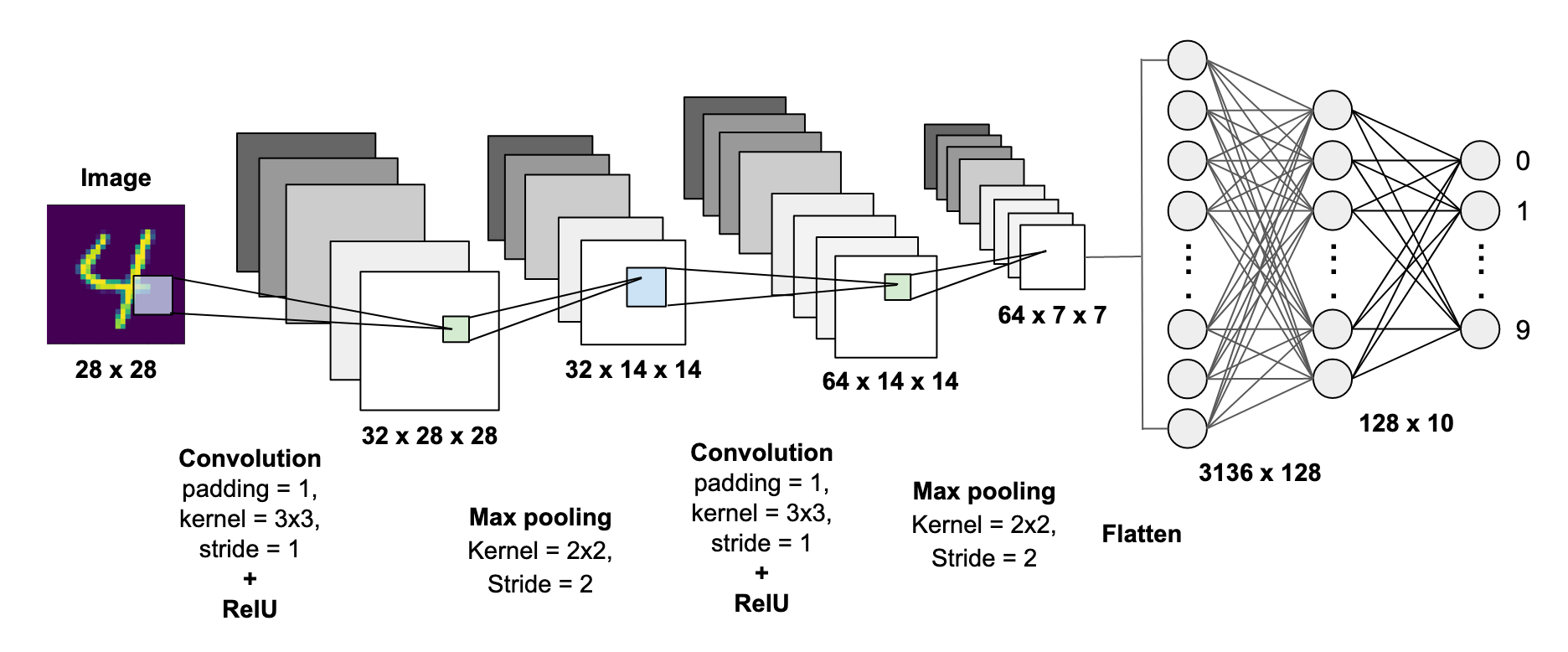
To begin developing the Convolutional Neural Network, we first need to import the required functions from the Keras ML library. The CNN architecture is then defined using a series of the model.add function. The architecture for this project contains:
- 2 Convolutional Layers, both of which have a 3 x 3 convolutional window and ReLU activation function. The first Conv layer produces 200 feature maps, whereas the second produces 100 feature maps. Stride and Padding has not been altered in this project.
- 2 Max Pooling layers, both of which have window sizes of 2 x 2.
- 2 Fully-Connected layers (one hidden layer, one output layer). The hidden layer has 50 neurons, and the output layer has only 2 (one for each class). Softmax activation function has been used to calculate the class probabilities.
- The model also uses dropout to help prevent overfitting of the model to the training data. More information on this hyper-parameter can be accessed here.

As with every machine learning implementation, the dataset is split into ‘training’ and ‘testing’ subsets. Here, 90% of the data is used to train the model, and 10% is used to test the model.

The model trains for 20 epochs with the loss and accuracy communicated through the programming interface. 20% of the data is used to validate the model. The best performing model is saved into a project file. As you can see, by epoch 11 the model was able to hit over 99% accuracy and under 0.03 loss on the training data.

The loss value for each epoch of training is plotted in the graph above. From about epoch 7 onwards, the loss continues to decrease on the training set, but not on the validation set. This is a sign that the model is starting to overfit to our training data. There are a number of alterations that could be made to help counteract overfitting, however, as we’ll see from below, the model still manages to achieve an impressive accuracy score on the validation data without these alterations in place.

Along with plotting the model’s loss over each epoch, we also plot the model’s accuracy score. This metric tends to average out at about 97% on the validation set, which is an impressive score for the size of the dataset we used to train the model. Testing the model on the actual unseen test data set yielded an accuracy score of 97.71% with a loss of 0.07.
4. Model deployment for live webcam feeds

Now that the model has been trained and it’s performance has been evaluated on the unseen images from the test set, we can think about how we want to feed our live webcam images into the model for prediction, and how we would like the prediction to be fed back to the user in a suitable format. All of the images from the webcam feed will need to undergo the same data pre-processing steps that we carried out on the training data, with the additional step of identifying where a face is located within the webcam image. The visual above shows how the webcam feed will be processed from the original image to a cropped “face only” image, to the fully pre-processed image ready for classification.
In terms of the visual feedback from the classification task, we have decided that the output will come in the form of two rectangular boxes (one will have a Green outline if a mask is present, and a Red outline if a mask is not present) and the other will encompass the Class label (‘Mask’ or ‘No Mask’). These boxes will be shown on the live webcam feed around our cropped “face only” image.


We first use Cv2.CascadeClassifier (Haar Cascade Frontal Face) to detect faces within an image. This classifier is a very popular algorithm that can be used to detect single or multiple faces within the image. To learn more about this, you can visit this webpage.
Cv2.VideoCapture(0) indicates that we would like to capture video data from the device’s camera. For this project, I have used the built-in Apple Mac webcam.
I have then defined the labels dictionary (Mask or No Mask) and the colour dictionary (Red if No Mask, Green if Mask).
While the webcam feed is live, we used source.read() to take in each individual image from the video, we then use Cv2.cvtColor to convert the image from an BGR image to a Grayscale image, and then split all the detected faces out into their individual items of data.
For each x,y co-ordinate, and width and height of the detected faces, we crop the image to include just the face only and then resize it dimensions to 100 x 100 which is the same as our training images. We also convert this to a numpy array and then divide all pixel values by 255 to normalise the pixel value range.
The image has now been fully prepared and is ready to be classified by the algorithm. model.predict is the line of code that evaluates the image and receives a classification decision. The visual rectangle feedback and output label is chosen based on the classification result, and this is overlayed on the webcam feed (as shown below).


— — — — — — — — —
Like this content? Please consider following me and sharing the story! Kindly drop any questions or comments below and I’ll get back to you. Thank you & have a great day :)
Reach out to me on LinkedIn: https://www.linkedin.com/in/thomas-staite-msc-bsc-ambcs-55474015a/
References
“A Comprehensive Guide to Convolutional Neural Networks — the ELI5 way” Sumit Saha, 2018. Available from < https://towardsdatascience.com/a-comprehensive-guide-to-convolutional-neural-networks-the-eli5-way-3bd2b1164a53 > [accessed on 15/08/2020]
“Face Mask Detection Keras” Thakshila Dasun, 2020. Available from <https://github.com/aieml/face-mask-detection-keras> [accessed on 16/08/2020]
