In the series of small articles, we will write step-by-step a toy text-to-speech model. It will be a simple model with a modest goal — to say “Hello, World”. This part focused on train set, audio transformations and dataloader.
Full source code: https://github.com/tttzof351/SimpleTransfromerTTS
Let’s run to the very end and see what we get:
What exactly are we going to do?
We will write a transformer-based autoregressive acoustic model using torch/torchaudio, inspired by the article https://arxiv.org/abs/1809.08895 (but with some simplifications).
Train set
We will use LJSpeech — 13K text-to-voice pairs from one speaker, with an average duration of utterance of ~7 seconds and full sizes in ~2.6 Gb.
Example:
The examination and testimony of the experts enabled the Commission to conclude that five shots may have been fired,
There are some gaps in the LJSpeech source files, so we will take the version from kaggle:
- Wavs: https://www.kaggle.com/datasets/mathurinache/the-lj-speech-dataset
- Metafiles: https://www.kaggle.com/datasets/tttzof351/ljspeech-meta
Text transformation
Before training, the text needs to be normalized — open abbreviations, convert all numbers into words, etc. Authors of LJSpeech have already done this operation. Next, you need to break the text into elements and there are options:
- Use letters — the most obvious way
- Use phonemes — split the text into phonemes, elements corresponding to the pronunciation. Phonemizers are used for this (espeak-phonemizer, g2p_en)
We will use the first option again — solely for the sake of simplification.
Let’s start to write code! First, create a hyperparams.py to store the constants:
class Hyperparams:
  seed = 42

  # Paths to datasets, dir for logs, for save steps
  csv_path = "/content/metadata.csv"
  wav_path = "/content/LJSpeech-1.1/wavs"
  save_path = "/content/gdrive/MyDrive/Colab Notebooks/params"
  log_path = "/content/gdrive/MyDrive/Colab Notebooks/train_logs"

  save_name = "SimpleTransfromerTTS.pt"

  # Alphabet
  symbols = [
    'EOS', ' ', '!', ',', '-', '.', \
    ';', '?', 'a', 'b', 'c', 'd', 'e', 'f', \
    'g', 'h', 'i', 'j', 'k', 'l', 'm', 'n', 'o', 'p', 'q', \
    'r', 's', 't', 'u', 'v', 'w', 'x', 'y', 'z', 'à', \
    'â', 'è', 'é', 'ê', 'ü', '’', '“', '”' \
  ]

...
The text transformation would then look like (text_to_seq.py):
import torch
from hyperparams import hp

symbol_to_id = {
  s: i for i, s in enumerate(hp.symbols)
}

def text_to_seq(text):
  text = text.lower()
  seq = []
  for s in text:
    _id = symbol_to_id.get(s, None)
    if _id is not None:
      seq.append(_id)

  seq.append(symbol_to_id["EOS"])

  return torch.IntTensor(seq)
We just used a fixed dictionary, skipping any missing characters. And at the end, they added the symbol EOS — end of the sequence.
print(text_to_seq("Hello, World"))Out:
tensor([15, 12, 19, 19, 22, 3, 1, 30, 22, 25, 19, 11, 0], dtype=torch.int32)Audio transformations. Theory
Usually a large number of transformations are required before we can use audio in training. It would be naive to attempt to reveal them in detail in small article. If this is a new topic for you, then I send you to a wonderful series of lectures:
So, next will be my trying of short brief explanation:
We start by saying that audio is dependency of amplitude versus time f(time) ⭢amplitude.
Let’s show it:
#load wav
wav_path = f"{hp.wav_path}/LJ001-0001.wav"
waveform, sample_rate = torchaudio.load(wav_path, normalize=True)

#plot wav
_ = plt.figure(figsize=(8,2))
_ = plt.title("Waveform")
_ = plt.plot(waveform.squeeze(0).detach().cpu().numpy())
_ = plt.xlabel("Time")
_ = plt.ylabel("Amplitude")
Short-time Fourier transform — STFT
But we also know that using the frequency domain allows us to analyze the signal more “deeply” using for this fast fourier transform (FFT). Why is it so — good question, I like this explanation.
Using FFT we get the dependence of power versus frequency g(frequency) ⭢power. But we’ve lost time! And we know that time is important — speech is divided into words and sentences.
The obvious way to combine the two approaches (time and frequencies) using window transformation which called short-time fourier transform (STFT).

MEL scale
Not all frequencies are equally perceived by human hearing. This opens up ways to reduce the dimensionality of the signal — removing little useful frequencies. For all this he uses Mel-scale transformations.
Griffin-Lim algorithm
Using for learning spectrograms we also achieve from model spectrograms. For reconstruction audio from spectrogram can take two approaches:
- Vocoders — separate NN model. See: https://docs.nvidia.com/tao/tao-toolkit/text/tts/vocoder.html
- Griff-Lim — phase reconstruction method based on the redundancy of the short-time Fourier transform.
Audio transformations. Code
In practice we will use torchaudio — official pytorch library for signal processing. All of the above transformations are already implemented there and are available for use with one line of code.
- torchaudio.transforms.Spectrogram — wrap around STFT
- torchaudio.transforms.MelScale — convert normal STFT into a mel frequency STFT
Torchaudio contains wonderful diagram shows links between different transformation. I used red for showing of preparation the audio to use in training, and in blue are the ones we’ll use to get the sound in the inference stage:

Write to all transformations
STFT melspecs.py#L7
from melspecs import spec_transform

# wav -> spectrogram-power
spec = spec_transform(waveform)

# Plot spectrogram-power
fig, (ax1) = plt.subplots(figsize=(4, 4), ncols=1)

_ = ax1.set_title("Spectrogram power")
pos = ax1.imshow(spec.squeeze(0).detach().cpu().numpy())
_ = fig.colorbar(pos, ax=ax1)

_ = ax1.set_xlabel("Time")
_ = ax1.set_ylabel("Frequency")
The problem is visible here — in this form, the data is visually poorly distinguishable (look at the lower frequencies — something is still visible there). This means that when training the model, it will be difficult to learn to distinguish between individual parts of the data and identify patterns.
In addition, it is clear that most of the data is empty — this is a consequence of the fact that only a narrow part of the frequencies is significant.
Next MelScale melspecs.py#L7
from melspecs import mel_scale_transform

# spectrogram-power to mel-spectgrogram-power
mel_spec = mel_scale_transform(spec)

# Plot mel-spectgrogram-power
fig, (ax1) = plt.subplots(figsize=(8, 3), ncols=1)

_ = ax1.set_title("Mel-Spectrogram power")
pos = ax1.imshow(mel_spec.squeeze(0).detach().cpu().numpy())
_ = fig.colorbar(pos, ax=ax1)

_ = ax1.set_xlabel("Time")
_ = ax1.set_ylabel("Frequency")
We have reduced the data dimension, but it is still a poorly distinguishable image. The reason for this is that the absolute energy difference at different frequencies is not so great. To make the difference more pronounced, a transition to decibels is used.
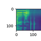
Apply power to db transformation melspecs.py#L47
from melspecs import pow_to_db_mel_spec

# mel-spectrogram-power to mel-spectrogram-db
db_mel_spec = pow_to_db_mel_spec(mel_spec)

# Plot mel-spectrogram-db
fig, (ax1) = plt.subplots(figsize=(8, 3), ncols=1)

_ = ax1.set_title("Mel-Spectrogram db")
pos = ax1.imshow(db_mel_spec.squeeze(0).detach().cpu().numpy())
_ = fig.colorbar(pos, ax=ax1)

_ = ax1.set_xlabel("Time")
_ = ax1.set_ylabel("Frequency")
Well — it looks like what you need! Lots of detail with a relatively small amount of data. Of course, this chain of transformations comes with a loss of information. The composition of the transformations will look predictable:
def convert_to_mel_spec(wav):
  spec = spec_transform(wav)
  mel_spec = mel_scale_transform(spec)
  db_mel_spec = pow_to_db_mel_spec(mel_spec)
  db_mel_spec = db_mel_spec.squeeze(0)
  return db_mel_spec
Now let’s do the reverse transformations and compare them with the original file to see if we’ve lost something important.
Original:
IPython.display.Audio(waveform, rate=hp.sr)The inverse transformation is based on the Griffin-Lim transformation we have already discussed.
from melspecs import inverse_mel_spec_to_wav

# mel-spec-db -> waveform
pseudo_wav = inverse_mel_spec_to_wav(db_mel_spec.cuda())

IPython.display.Audio(
    pseudo_wav.detach().cpu().numpy(),
    rate=hp.sr
)
Inversed:
Dataset/Dataloader
Now we can write a class to load data by combining text and sound transformations. It will simply return a text/utterance pair after transformations
class TextMelDataset(torch.utils.data.Dataset):
    ...

    def get_item(self, row):
      wav_id = row["wav"]
      wav_path = f"{hp.wav_path}/{wav_id}.wav"

      text = row["text_norm"]
      text = text_to_seq(text)

      waveform, sample_rate = torchaudio.load(wav_path, normalize=True)
      assert sample_rate == hp.sr

      mel = convert_to_mel_spec(waveform)

      return (text, mel)

    ...
Now, to complete the formation of the dataset, we need to combine individual samples into batches. At the same time, our model allows us to use an arbitrary size for the dimension responsible for the length of the text and audio. This allows you to use just the maximum size in the single batch for alignment. This is more efficient than choosing the maximum size for the entire dataset and aligning the samples to it.

def text_mel_collate_fn(batch):
  # Find max len of text in batch
  text_length_max = torch.tensor(
    [text.shape[-1] for text, _ in batch],
    dtype=torch.int32
  ).max()

  # Find max len of mel spec in batch
  mel_length_max = torch.tensor(
    [mel.shape[-1] for _, mel in batch],
    dtype=torch.int32
  ).max()


  text_lengths = []
  mel_lengths = []
  texts_padded = []
  mels_padded = []

  for text, mel in batch:
    text_length = text.shape[-1]

    # Alignment text with max text
    text_padded = torch.nn.functional.pad(
      text,
      pad=[0, text_length_max-text_length],
      value=0
    )

    mel_length = mel.shape[-1]

    # Alignment mel-spec with max mel-spec
    mel_padded = torch.nn.functional.pad(
        mel,
        pad=[0, mel_length_max-mel_length],
        value=0
    )

    # Keep original text lens
    text_lengths.append(text_length)

    # Keep original mel-spec lens
    mel_lengths.append(mel_length)

    # Keep alignmented text
    texts_padded.append(text_padded)

    # Keep alignmented mel-specs
    mels_padded.append(mel_padded)

  text_lengths = torch.tensor(text_lengths, dtype=torch.int32)
  mel_lengths = torch.tensor(mel_lengths, dtype=torch.int32)
  texts_padded = torch.stack(texts_padded, 0)
  mels_padded = torch.stack(mels_padded, 0).transpose(1, 2)

  # New element - STOP token
  # Needed to learn when to stop generating audio.
  gate_padded = mask_from_seq_lengths(
      mel_lengths,
      mel_length_max
  )
  gate_padded = (~gate_padded).float()
  gate_padded[:, -1] = 1.0

  return texts_padded, \
         text_lengths, \
         mels_padded, \
         gate_padded, \
         mel_lengths
Let’s check batch’s structure.
df = pd.read_csv(hp.csv_path)
dataset = TextMelDataset(df)

train_loader = torch.utils.data.DataLoader(
    dataset,
    num_workers=2,
    shuffle=True,
    sampler=None,
    batch_size=hp.batch_size,
    pin_memory=True,
    drop_last=True,
    collate_fn=text_mel_collate_fn
)

def names_shape(names, shape):
  assert len(names) == len(shape)
  return "(" + ", ".join([f"{k}={v}" for k, v in list(zip(names, shape))]) + ")"

for i, batch in enumerate(train_loader):
  text_padded, \
  text_lengths, \
  mel_padded, \
  mel_lengths, \
  stop_token_padded = batch

  print(f"=========batch {i}=========")
  print("text_padded:", names_shape(["N", "S"], text_padded.shape))
  print("text_lengths:", names_shape(["N"], text_lengths.shape))
  print("mel_padded:", names_shape(["N", "TIME", "FREQ"], mel_padded.shape))
  print("mel_lengths:", names_shape(["N"], mel_lengths.shape))
  print("stop_token_padded:", names_shape(["N", "TIME"], stop_token_padded.shape))

  if i > 0:
    break
Out:
=========batch 0=========
text_padded: (N=32, S=152)
text_lengths: (N=32)
mel_padded: (N=32, TIME=841, FREQ=128)
mel_lengths: (N=32)
stop_token_padded: (N=32, TIME=841)
=========batch 1=========
text_padded: (N=32, S=153)
text_lengths: (N=32)
mel_padded: (N=32, TIME=864, FREQ=128)
mel_lengths: (N=32)
stop_token_padded: (N=32, TIME=864)- N — batch size
- S — text size
- TIME — time size for the spectrogram
- FREQ — frequency size
Stop token
Because our model is autoregressive — need to learned moment to stop generate audio. For this using stop_token — just tensor with length by time like alignmented spectrogram and contains 0 while signal contains information (not-allignment part) and 1 when signal contains zeros (alligment part). Like this:
tensor([0., 0., 0., ..., 1., 1., 1.])
This part is end. Dataloader is finished to train model. The next part will be the implementation of the model itself.
Model

Simplifications:
- No Text-to-phone convertor
- Instead Scaled Encoding using simple Embedding Encoder
Code: model.py
The moment which I want to highlight: the use of a dropout in the DecoderPreNet, not only during the training process, but also during the inference.
class DecoderPreNet(nn.Module):
  def __init__(self):
    super(DecoderPreNet, self).__init__()
    self.linear_1 = nn.Linear(
      hp.mel_freq,
      hp.embedding_size
    )

    self.linear_2 = nn.Linear(
      hp.embedding_size,
      hp.embedding_size
    )

  def forward(self, x):
    x = self.linear_1(x)
    x = F.relu(x)

    x = F.dropout(x, p=0.5, training=True)

    x = self.linear_2(x)
    x = F.relu(x)
    x = F.dropout(x, p=0.5, training=True)

    return x
This explains the need to keep variance of data which we use in decoder and used in Tacotron2.
https://arxiv.org/pdf/1712.05884.pdf: In order to introduce output variation at inference time, dropout with probability 0.5 is applied only to layers in the pre-net of the autoregressive decoder.
Train