Experience the magic of Generative Adversarial Networks

In this post, we discuss the details behind our GAN demo at RealityEngines.AI.
Generative adversarial networks (GANs) are viewed by many as the most exciting deep learning development of the last decade, with many applications including data augmentation, image generation, image completion, and image editing. In this post, we explain how we use GANs to change the emotion, age, and gender of any uploaded photo of a human face, or even a famous painting such as Alexander Hamilton on the ten dollar bill or the Mona Lisa.

The demo also outputs a video of the uploaded image talking out a prompt.


Our demo makes use of cutting-edge deep learning techniques such as StyleGAN, InterFaceGAN, and ATVGnet. It uses several other deep learning models as subroutines. In fact, the algorithm uses seven different neural networks each time you upload a new image. We will start with a high-level overview before we get into the details of the techniques.
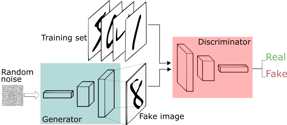
At the heart of the algorithm is a GAN. While standard neural networks can classify images, e.g. distinguishing between cats, dogs, and other animals, GANs can generate new images, e.g. creating new images of human faces that do not exist. GANs use two neural networks: a generator and a discriminator. The goal of the generator is to create new images that look similar to the training data. The goal of the discriminator is to distinguish between real images (from the training data) and fake images (from the generator). The generator and the discriminator compete against each other during training — the generator tries to fool the discriminator, and the discriminator tries not to get fooled by fake images. To make sure the generator does not output the same image every time, it takes as input a set of random numbers (a latent vector) and it uses these numbers to make decisions about the face such as hair and eye color.
In fact, at RealityEngines.AI, we use GANs for data augmentation as well as our face demo. We describe our techniques for the demo and data augmentation below.
Emotion Editing
To explain how we change the emotion of an image, imagine that we are baking cookies. A new batch comes out of the oven, and we decide that they need more chocolate chips. It would be quite challenging to add chocolate chips directly to this batch of cookies, but if we start a new batch, we can add more chocolate chips to the ingredients. This is the same for GANs — it is very hard to change the emotion of a face directly on the image (after it is generated), but we can change the latent vector before it is generated.

Say we want the cookies fluffier, and we don’t know whether that is controlled by baking powder, flour, or something else. What we can do is run an experiment. We bake many batches of cookies with different combinations of ingredients, and we see which ones come out fluffy and which ones don’t. Now it is easy to see that baking powder was the key, so we can make any new recipe fluffier by adding more baking powder while keeping all other ingredients the same. This is what we do in the demo. We generate many faces, (or use a dataset of faces), label the faces as happy or not happy, and then run a classifier on the latent vectors. What we get is an emotion vector. We can add this vector to any new latent vector to make the corresponding image happier without changing any other attributes of the person.
When a new image is uploaded, we convert the image into a latent vector, add the emotion vector, and convert the new vector back to an image. Later in this post, we go into more technical detail assuming a deep learning background.
Data Augmentation
At RealityEngines.AI, we also use GANs for dataset augmentation (see this post or this talk). We build upon the recent Data Augmentation Generative Adversarial Network (DAGAN). A DAGAN is a technique for meta-learning or transfer learning: we train the DAGAN on a source domain, for which we have enough data, and then generate synthetic data on a target domain, for which we may not have enough data. This approach has been shown to significantly improve classification performance in the target domain. We have tested the DAGAN on the Omniglot and Fruit360 datasets. For example, the source domain may consist of images of letters from the English alphabet, while the target domain consists of Japanese characters.

In a standard GAN, the goal of the generator is to generate new, realistic images which are similar to the training data. In the DAGAN, the goal of the generator is to augment each training datapoint without changing the label of the datapoint. The discriminator then takes in pairs of points as inputs — either a datapoint and its generated augmentation, or two random datapoints from the same class, and tries to tell the different types of pairs apart.

We improve the DAGAN by using neural architecture search (NAS) guided by the classification performance of a neural network in the target domain. Our work represents one of the few approaches in applying NAS to GANs, since GANs are hard to train. In addition, there is no universally accepted performance metric for GANs that a NAS system can use to guide its search.
Video Generation
To generate a video of the image talking out a prompt, we use a separate pipeline, the ATVGnet, which takes in an audio sample in addition to the image. This pipeline has two steps performed by two different networks: the audio transformation network (AT-net) and the video generation network (VG-net). In the first step, the AT-net takes in the audio sample and converts it into a set of facial landmarks — e.g., locations of a nose, eyes, ears, lips, etc. In the second step, the VG-net takes in the image of the face, along with the landmarks we generated in the first step, and imposes the landmarks onto the face. We do this for each set of landmarks, which results in a video.

The figure above shows the AT-net in action. The AT-net takes in an audio signal containing speech and an image of a face and produces a sequence of landmarks. These correspond to the person in the input image voicing the audio signal. Both the AT-net and the VG-net make use of recurrent neural networks (RNNs) to ensure that their outputs remain consistent across time. The AT-net uses an LSTM (Long short-term memory) module. LSTMs are a variant of RNNs that can process long sequences of data without running into problems that vanilla RNNs usually face. At the core of the AT-net, we have an LSTM that takes in as inputs encodings of the principal components of facial landmarks, encodings of the audio signal, and the LSTM’s input from the previous time step. It predicts the landmarks.

The figure above shows the VG-net in action at a high level. The VG-net takes in as inputs: (1) the sequence of landmarks from the AT-net ; (2) the input image; and (3) the landmarks for the input image. The VG-net operates on the assumption that the difference between the AT-net’s predicted landmark and input landmark (Step A) corresponds to the distance in pixel space between the input image and desired output frame. Based on this assumption, using a multi-modal convolutional RNN (MMCRNN), we compute a motion map (Step B). Since the MMCRNN is a recurrent network, the output from the previous time step is fed in as input to the next time step. This ensures that frames are consistent across time. We also compute an attention map (Step C) based on the difference between the predicted and input landmarks. This attention map is then used to combine the motion map with the input image to produce the final frame at time t (Step D).
Please adhere to our Terms of Service and Privacy Policy when uploading your image. At RealityEngines.AI, we do our best to remove bias from deep learning models, but there is a possibility that the demo output will contain bias inherent in the training dataset.
Under the Hood
For the rest of this post, we will go into more of the details of the algorithms that make up the demo.
Our algorithm makes use of the pre-trained, publicly available StyleGAN, which was trained on a dataset of 70,000 high-quality headshot photos from Flickr, needing thousands of GPU-hours to train. We use the fully trained generator network from StyleGAN, which is a function that maps latent vectors to human faces.
Face editing
Another recent research paper, InterFaceGAN, showed how to change the gender or age of images generated from a GAN. The idea is to generate thousands of human faces using StyleGAN, and then classify features such as age or gender. We can then train a linear classifier in the latent space using a support vector machine. Once we learn a linear decision boundary for a feature such as younger than 40 or over 40, we compute the normal vector to the decision boundary. Given any latent vector of a person who is under 40, we can add the normal vector to increase the age of the person while keeping all other features constant.
Inverting the generator
So, now we know how to edit images generated by the StyleGAN, but what if we want to edit specific images, such as the Mona Lisa? The StyleGAN image space is rich enough to contain images virtually identical to the Mona Lisa, but how do we find the corresponding latent vector? Recent advancements have made this possible. We guess a latent vector, and then use backpropagation through the StyleGAN using the distance between our guess and the real Mona Lisa computed with features from the middle layer of a VGGNet trained on ImageNet. However, by itself, the backpropagation would take too long. Before running gradient descent, we can use an EfficientNet trained to map images to latent vectors, to get a good initial guess of the latent vector. This substantially decreases the runtime of gradient descent.
Computing emotion vectors
Now with a pipeline for computing the latent vector of any image, we can convert whole datasets of faces into latent vectors. This is exactly what we did — we converted 4,000 images from the Cohn-Kanade AU-Coded Expression Database into latent vectors. We used an emotion classifier to label the images with emotion, and we use an SVM to classify the corresponding latent vectors. Then the normal of the decision boundary gives us emotion vectors for anger, happiness, fear, etc. Adding one of these vectors to any latent vector exaggerates the corresponding emotion.
We use new techniques to improve the quality of the emotion vectors. We use an SVM classifier on the mapping network vectors (18x512) instead of the latent vectors (1x512), and we use vector projection to further isolate out certain traits.
ATVGnet
For the video generation network, as described above, we use a separate pipeline based on a state-of-the-art architecture, the ATVGnet (with two components: AT-net and VG-net), that generates talking faces from a single image and audio sample. This architecture is based on a cascaded GAN architecture. A trained ATVGnet takes as input an image of a person p, and a voice sample a (that can be from some other person) and generates a video of p voicing the voice sample a. Training the ATVGnet is done using videos of people talking. Rather than producing a video directly from the input audio as in previous approaches, the ATVGnet has two steps. We briefly go through the steps below.
In the first step, the AT-net takes as input a person p’s image ip, face landmarks of p given by Lp and an audio sample <a1…aT>, and produces a sequence of face landmarks <q1…qT> corresponding to what the person’s facial landmarks would be if that person were to voice the audio. This happens as follows. Given the audio signal, the AT-net first computes the Mel-frequency cepstral coefficients (MFCC) of the audio signal. MFCCs are commonly used in audio and speech processing. Then we pass the MFCC of the audio signal through an encoder network to get a representation that we then use for processing. AT-net also takes in the facial landmarks of the input image (computed outside of ATnet). We then compute the principal components of the landmarks and then pass the principal components through an encoder. Then at the core of the AT-net, we have an LSTM module that at time t takes in as inputs (1) encodings of the principal components of the landmarks; (2) encodings of the MFCC of the audio signal; and (3) the LSTM’s output from the previous time step and predicts the landmarks at time t. Output from the LSTM module are then passed through a decoder and a PCA reconstruction module to recover the predicted landmark for the video at time t. Authors of ATVGnet observe that using PCA components for the landmarks helps in reducing facial movements that are not related to the audio signal.
In the second step, the VG-net takes the landmark sequence <q1…qT>, input image ip and its landmarks Lp and produces a sequence of image frames <v1…vT> corresponding to the landmark sequence. This gives us our final video. We explain briefly how this happens. For the VG-net, the inputs are: (1) the sequence of landmarks from the AT-net ; (2) the input image; and (3) the landmarks for the input image. At time t, the VG-net computes the difference d between the AT-net’s predicted encoded landmark and encoded input landmark. The VG-net operates on the assumption that the difference between the AT-net’s predicted landmark at time t and input landmark corresponds to the distance in pixel space between the input image and desired output frame at time t. The difference d is then combined with an encoding of the input image to produce a frame feature (v). The frame feature is then fed into a multi-modal convolutional RNN (MMCRNN) to compute a motion map m. Since MMCRNN is a recurrent network, we also have as input at time t, an output from time t — 1. This ensures that frames are consistent across time. We then compute an attention map a based on the predicted encoded landmark and encoded input landmark. This attention map is then used to combine the motion map with the input image to produce the final frame vt at time t: vt = m * a + (1-a) * ip.
One of the innovations of ATVGnet over prior approaches is in using an attention mechanism in the VG-net to generate the frames. This attention mechanism reduces irrelevant motion in the output video. We modify the pipeline in two ways. We retrain an existing model with new data with improved preprocessing, and we also modify the attention process in VG-net to reduce unnecessary movement in the output video.
Written by Colin White and Naveen Sundar Govindarajulu.