AI Saturdays Bangalore Chapter: Everything about Convolutions (Week 6)

After 5 Saturdays of covering the basic concepts required for understanding any modern deep architecture, it was time. Week 6 was all about the convolutions; from basic concepts like stride and padding to building our own deep architecture while reasoning on why a specific hyperparameter was chosen.
This week, we covered the contents of Fast.ai Lesson 3. Apart from the solid introduction to convolutions, Lesson 3 also talks about multi-label classification and how one can use Fastdotai library on a Kaggle competition namely, Planet: Understanding Amazon from the space. So, the post-lunch session was all about understanding the code and running the Kaggle kernel.

We all know Convolution Neural networks (the second generation neural networks) opened the Pandora box that helped us solve all those problems easily which were once thought to be very hard to solve.
So, what is this Convolution Neural network(CNN)?
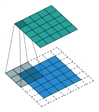
In layman terms, it’s a stack of convolution layers with a mix of other types of layers which we will look into it soon. A single convolution layer looks like follows:

The blue grid is the input to the convolution layer. The darker area that’s sliding over the input is called the filter or kernel. When the filter/kernel is slid over the input in a particular way, it produces the green grid known as the feature map.
This act of producing a feature map using a kernel and an input image is called convolution. Let’s take a look at the math on how a feature map is produced.

When a kernel is slid over the input, it multiplies the corresponding values and sums them up. This is done until the kernel reaches the end of the image. When all the resulting outputs of the convolutions are arranged as shown, we get the feature map. In CNNs, the convolutions layers are stacked one upon other. So, the produced feature map at one layer becomes the input to the next convolution layer.
The filter can be slid on an input in many ways. So, which is the right way? Well, there is no one right way as it is a hyperparameter which can be chosen by us or change them and observe whichever gives the best performance. Mainly, there are 3 hyperparameters when it comes to convolution layer: Filter/Kernel size, Stride and Padding.
Filter/Kernel size: It is the dimension of the filter. For example, when size=3, it means the kernel dimension is 3x3. We choose the kernel size based on the characteristics of the input. If we want to have a larger receptive field, ie., the kernel should be able to look at a bigger chunk of the input image, we go for a higher odd number sized filter.
One might wonder why is the size of the filter/kernel odd. That is because convolution is all about getting the correlation among a central pixel and it’s neighboring pixels. So, if we take an even sized kernel, there will not be any central pixel and we would miss the intuition/point of convolution. Mathematically, it will work but conceptually, it is not intuitive.
Stride: It’s the number of steps the filter/kernel is moved during convolution. In images, the number of steps is the number of pixels. Can you spot the difference?

So, why do we want different strides? If the data is sparsely located in the image, the filter/kernel can slide over the input quickly as much information isn’t present anyways. Similarly, if the information is dense, a small stride is desired. Usually, stride=1 is the default. Do you know another reason? Post it in the comment section. :)


Padding: It means adding extra pixels around the boundary or pad the image.
We use padding for many reasons. Here are a few:
- When a series of convolutions are performed, the produced feature map keeps decreasing. At one point, we will not be able to apply any more convolutions and the network wouldn’t be as deep as required. To avoid this situation, we pad the produced feature map which will result in a deeper network.
- Also, when convolutions are applied, the information in the borders is lost. To avoid this, one can pad the input.
Pooling layers:
There are also other non convolution layers like pooling layer. As the name suggests, this layer picks a value from a pool of values. The commonly used pooling layer is maxpooling. Given the pooling filter size, it chooses the max value from the pool of the specified filter size.

On the other hand, average pooling outputs the average of the pool. And minpool is the opposite of maxpool. So, the question arises of when to use what. A superb example from fast.ai course on difference between maxpooling and average pooling:
In classifying cats vs. dogs, averaging over the image tells us “how doggy or catty is this image overall.” Since a large part of these images are all dogs and cats, this would make sense. If you were using max pooling, you are simply finding “the most doggy or catty” part of the image, which probably isn’t as useful. However, this may be useful in something like the fisheries competition, where the fish occupy only a small part of the picture.
Activation functions:

As Jeremy mentions in his lectures, each activaion function has it’s own charecteristics. Depending on the kind of our necessity, we choose the activation. Let’s consider the case of single label prediction v/s multi-label prediction. In a problem of predicting only a single value, we would be using softmax activation because softmax kind of highlights the max value while supressing lower values. This way, it created a better margin between the max predicted and other predicted values while maintaing the sum of all prediction equal to 1. But in the case multi-label prediction, there might be a case where multiple predictions are correct. In that case, we cannot use softmax because softmax would supress other predictions while keeping only the highest one. In this case, we go for sigmoid activation for each prediction that squashes the values between 0 and 1 and therefore denoting the probability of the prediction.
Building an Architecture:
While building the architecture, we need to have a better idea mainly on the number and dimension of feature maps produced. Two simple rules one needs to keep in mind are these:
1. Number of filters used on an input is equal to the number of feature maps produced
2. Dimension of the produced feature map is (N + 2P - F)/S + 1 where,
N : input size;
P : Padding;
F : Filter size;
S : Stride.
For example, is the input image is 28x28 and without any padding and a 3x3 filter with a stride of 1, we get a feature map of (28 + 2*0 — 3)/1 + 1 = 26.
Let’s take the same above example but this time, let’s take it with padding. If we calculate, we’d be getting the size of feature map equal to the input size. Hence, that proves the first point of why use padding.
Till now, we have looked at individual components of a deep CNN. Let’s look at the whole architecture and understand while applying the knowledge we gained till now on what’s going in the below architecture:

Starting from the lefthand side, we have a convolution layer C1 that uses 5x5 convolutions on input size of 55x55 that resulted in a feature map os size 27x27. We can see that the depth of produced feature maps is 256. That means, 256 filters were used in C1. Same goes on for C2 that produces 384 feaure maps of 13x13 dimension. But from layer C3 to C4, the size of feature map produced is equal to the input. That means, padding was used there.
Fastforwarding to the last layers, FC means fully connected. Here, the network uses 3 FC layers. As we know, FC layers are very good function approximators but they use individual weights making it harder to train. Whereas CNNs share their weights and are easier to train.(A small set of weights, eg: 3x3 filter uses 9 weights, are used for the whole image hence sharing the 9 weights. But in the case of FCNNs, each pixel of the input gets its own weight therefore becoming harder to train). So, a combination of CNNs and FCNNs are used here to make use of the good parts of both type of networks.
The number of nodes in the last layer of the network is equal to the number of labels. The network is trained in such a way that corresponding node of that label has higher value compared to other nodes.
Post-Lunch Session:
In the post-lunch session, we understood and executed this Kaggle notebook, which has been forked and modified a little from William Horton’s notebook. One point to highlight here is the use of sigmoid activation function. As this is a multi-label clasification problem, use of sigmoid is prefrered over softmax.
Participants response:
Participants from various backgrounds have participated in this session. The feedback from them was impressive. We mentors are encouraged by this response. We are glad that the participants found this session useful.

It is just wonderful to teach and share your experiences with others. Thank you AI Saturdays for this amazing platform. Looking forward for the future sessions.
Alvidha!
