Bank Data: Classification Part 1

Part 1 out of 4 will be short posts about the 4 different machine learning algorithms that were used on the bank data.
Random Forest
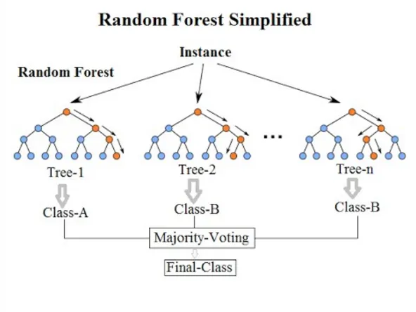
Random forest is an ensemble method that samples on a random subset of features and uses Bootstrap Aggregation (Bagging) to classify. Bagging is a sampling technique that samples with replacement of the data on each tree. We can then use Out of Bag Data, one thirds of the data left, to measure the performance of each tree, essentially testing the each tree on unseen data to measure the models performance.
from sklearn.ensemble import RandomForestClassifierrandom_forest = RandomForestClassifier(random_state=19, oob_score=True)# Random Forest grid search
param_forest = {"n_estimators":[300, 400], "max_depth":[5, 10, 15, 20]}
grid_forest = GridSearchCV(random_forest, param_grid=param_forest, cv=10)# Fitting training data to model
grid_forest.fit(X_train_new, y_train_new)
The code above shows use importing the Random Forest Classifier, instantiating, creating a grid search where the parameters that will be tuned are “n_estimators,” the amount of trees that will be splitting on a decision, and “max_depth,” how deep the tree will go, meaning more splits the denser the tree.
After fitting the model we can look at the best parameters and the cross validation results:

which shows us that we should get an accuracy score around 70% on our test data.
display(grid_forest.score(X_train_new, y_train_new))
display(grid_forest.score(X_test, y_test))
The code above gave horrible results that show an immense amount of Bias, under-fitting.
The training score showed a result of 93% while the test score showed 70%. Although this is a horrible accuracy score this is not what we completely care about.
Since our dependent variable is binary and we care about which characteristics do people have that pay off their loan in full, helping banks focus on which characteristics need to be strong in order to give a loan. This means that it’s best to use the confusion matrix, another performance metric for classification machine learning models.
Confusion Matrix
Why focus on confusion matrix and not accuracy or AUC ROC scores? This is because we have imbalanced data. If you can remember, we used SMOTE because our data was heavily imbalanced. SMOTE was used on our training data, so it makes sense why we are receiving bias results. Accuracy is telling us that our model predicted 93% of the points in the correct class, but it does not specify which. AUC ROC is also not a good idea to use on imbalanced data.
# Able to determine metrics for a confusion matrix
def confusion_matrix_metrics(TN:int, FP:int, FN:int, TP:int, P:int, N:int):
    print("TNR:", TN/N)
    print("FPR:", FP/N)
    print("FNR:", FN/P)
    print("TPR:", TP/P)
    print("Precision:", TP/(TP+FP))  # % of our positive predictions that we predicted correctly.
    print("Recall:", TP/(TP+FN))  # % of ground truth positives that we predicted correctly.
    print("F1 Score:", (2*TP)/((2*TP) + (FP + FN)))  # the harmonic mean of precision and recall and is a better measure than accuracprint('Confusion Matrix - Testing Dataset')
print(pd.crosstab(y_test, grid_forest.predict(X_test), rownames=['True'], colnames=['Predicted'], margins=True))

The code above shows a function that calculates TPR, TNR, FNR, FPR, Precision, Recall, and F1 Score.
These scores will help us determine if how the model is classifying the data:

The image above shows us how the model did at classifying the positive (1) points.
Feature Importance
We can see what features were important to the model:
# Graphing
fig, ax = plt.subplots(figsize=(15, 10))
ax.barh(width=rf_clf.feature_importances_, y=X_train_new.columns)
The code above provided a visualization of our machine learning model deciding what features are more important than others, the higher the score, the more important those features are. From this, we will gain information on what is more important for banks to look at when deciding to give a loan to someone.
The graph above shows that there are many features that the Random Forest model categorized as important. We will have to give our best judgement on what we want our threshold to be in order to select the main important features:
# Selecting the top features at a cap of 0.05
top_important_features = np.where(rf_clf.feature_importances_ > 0.05)
print(top_important_features)
print(len(top_important_features[0]))  # Number of features that qualify# Extracting the top feature column names
top_important_feature_names = [columns for columns in X_train_new.columns[top_important_features]]
top_important_feature_names

The code above shows that we set our threshold greater than 0.5, and in return receive these features above as the more paramount ones.
Further Steps
We can also go a step further, we can take these features and create a new subset data with only these paramount features as our new independent variables, and then run them through our Random Forest grid search, view the cross validation results, and then run it through a confusion matrix to see how our model has performed with new important features.
I have already finished these steps and will just show the end results because that would be a lot of work to put them in this post.

The image above shows the results of our important features. It looks like we have a lower F1 score when using important features.
Why Random Forest?
Since this is the end I feel like this would be a good time to perform a Tarantino and explain the beginning. I use a Random Forest model because they are great with handling large binary data. Random forest is also great when preventing over-fitting, and I could also feed the model our raw, but purified data, allowing me to pass it through without feature scaling.