Deep Dive on YOLOv2 and YOLO9000
Better, Faster, and Stronger versions of the YOLO object detection model
The YOLO (You Only Look Once) object detection model brought out in 2015, was state-of-the-art among similar models of that time, boasting of astounding real-time prediction speeds (Fast YOLO could predict objects at 155 FPS (frames per second)) and an improved accuracy over previous models (YOLO did much better in detecting objects than models such as DPM and Zeiler-Fergus Faster R-CNN, high-performing models of that time).
While YOLO fared pretty well due to its faster detections and improved accuracies over previous models, it also had some shortcomings.
Relative to Fast R-CNN, a top-ranking model, YOLO makes a significant number of localization errors (8.6% compared to 19%)

Furthermore, it had a relatively low recall when contrasted with models which used region proposal-based methods (e.g. Faster R-CNN)
The creators of YOLO decided to fix these two main problems, while ensuring that the detection accuracy stays the same.
Introduction to YOLOv2 and YOLO9000
Redmon and Farhadi developed an improved version of YOLO, named YOLOv2, which had several features not seen in YOLO, such as multi-scale training (training on images of different resolutions), thus providing an easy trade-off between speed and accuracy.
They also proposed a novel method by which they could train the model simultaneously on both object detection and image classification datasets, thus bridging the gap between these two kinds of datasets (we’ll look at this below).
It takes two to tango, and in the same paper, the authors also talked about another model, YOLO9000, a real-time object detection model which can detect over 9000 object categories!
Trained jointly on both object detection and classification datasets, YOLO9000 can predict detections for object classes that don’t even have labeled detection data, and this model gives a nice performance on the ImageNet detection task.
Sounds interesting? Let’s take a deep dive below.
Better than YOLO
As we looked earlier, YOLO makes a larger number of localization errors compared to Fast R-CNN, and it’s recall is low when matched with region proposal based methods. In YOLOv2, the main concern was fixing these errors while maintaining the detection speed and accuracies.
The authors utilized a variety of concepts learned from field knowledge as well as some new techniques to result in a model which does better than YOLO. So, what are those techniques?
1. Batch Normalization (BN)
In simple terms, BN provides every layer of a neural network the capability to learn independently of other layers.
It normalizes the output of the previous activation layer by subtracting the mean of the batch and dividing by the standard deviation of the batch, & this output gets multiplied by a standard deviation parameter (gamma), then a mean parameter (beta) is added.

This process leads to notable changes in convergence and removes the need for other forms of regularization (such as dropout) without overfitting the model.
✅ When BN is added to all convolutional layers in YOLO, a
2% improvement in mAP (mean average precision) is observed.
2. High Resolution Classifier
YOLO trained the classification network at 224 x 224 image size and increased this to 448 x 448 for the detection process.
This results in the network switching to learning object detection in a short period of time and adjust itself to the new resolution.
In YOLOv2, the classification network is first trained on ImageNet at
224 x 224 resolution, then fine-tuned at the full 448 x 448 resolution for 10 epochs, on the ImageNet dataset, giving the network time to adjust its filters to work better on higher resolution input.
The final network is then fine-tuned on detection.
✅ This process of developing a high-resolution classification network results in an increase of around 4% mAP.

3. Convolutional with Anchor Boxes
YOLO predicts the bounding box coordinates directly using fully connected (FC) layers at the end of the model, on top of all convolutional layers (feature extractors).
Faster R-CNN has a better technique — using hand-picked priors (anchor boxes), it predicts offsets and confidences for these boxes at every location in a feature map. This simplifies the problem and makes it easier for the network to learn.
We can create 5 anchor boxes as follows.

We won’t predict 5 arbitrary bounding boxes, but predict the offsets constrained to the anchor boxes above. Doing this maintains the diversity of the predictions. The training of the model will be more stable.

If instead, we predict arbitrary bounding boxes for each object (like YOLO does), the training will be unstable, as our guesses might work well for some objects but not for others.

Thus, the changes we make to YOLO are listed below —
- Remove the FC layers at the end which predicted the bounding boxes, and use anchor boxes instead

2. Use input size of 416 x 416 instead of 448 x 448. Objects (especially large ones) usually occupy the center of the image, so for predicting these objects, a single location at the center would be better than 4 boxes close by. This step means our feature map will have a size of 13 x 13, because YOLO’s convolutional layers downsample images by a factor of 32.
Thus, an odd number of locations on our feature map would be better than an even number .

3. Decouple the class prediction mechanism from spatial locations and shift it to bounding box level.
For every bounding box, we now have 25 parameters — 4 for the bounding box, 1 box confidence score (called objectness in the paper), and 20 class probabilities (for the 20 classes in the VOC dataset).
We have 5 bounding boxes per cell, thus each cell will have 25 x 5, i.e. 125 parameters.
Similar to YOLO, the objectness prediction mechanism predicts the IOU (intersection over union) of the ground truth and the proposed box

We also remove one pooling layer to make the spatial output of the model
13 x 13, compared to 7 x 7 earlier.
✅Using anchor boxes decreases the accuracy to 69.2 mAP from 69.5, but results in a significant increase in recall, from 81% to 88%.
4. Dimension Clusters
This method suggests running K-means clustering on the training set bounding boxes to automatically find good priors, instead of starting with hand-picked anchor box dimensions.
We want priors that are independent of the bounding box size, so we use the following as our distance metric.
d(box, centroid) = 1 - IOU(box, centroid)The following figures show the result obtained by running K-means for various values of K and plotting the average IOU with the closest centroid. The authors note that K=5 offers a good trade-off between model complexity and high recall.
Relative centroids are shown for the VOC and COCO datasets. One thing common in both sets of centroids is the preference for tall, thin boxes than short, wide boxes. COCO has greater variation in size than VOC.

✅ The following table compares the average IOU to the closest prior of the clustering strategy and the predefined anchor boxes. Using K-means to generate the bounding boxes initializes the model with a better representation and makes the task easier to learn.

5. Direct Location Prediction
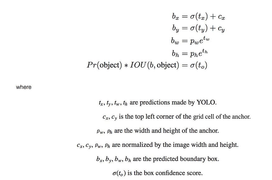
A problem that results from directly predicting (x, y) locations of the bounding box is model instability. What region proposal networks do instead is predict values tₓ and tᵧ and the (x, y) coordinates are calculated as follows
x = (tₓ * wₐ) - xₐ
y = (tᵧ * hₐ) - yₐ
Due to the offsets not being constrained here, any anchor box can end up at any point in the image, regardless of what location predicted it — the model takes a long time to stabilize for predicting sensible offsets.
An alternative is to predict location coordinates relative to the location of the grid cell, just like in YOLO. The network predicts 5 coordinates for every bounding box — tₓ, tᵧ, tཡ , tₕ, and tₒ, and a logistic function is applied to constrain the values of these coordinates to [0, 1]


This makes the network training more stable.
✅ The technique of dimension clusters and directly predicting the bounding box center location improves YOLO by ~5% over the version with anchor boxes.
6. Fine-Grained Features
Predicting detections on a 13 x 13 feature map works good for large objects, but for localizing smaller objects, finer-grained features might prove useful.
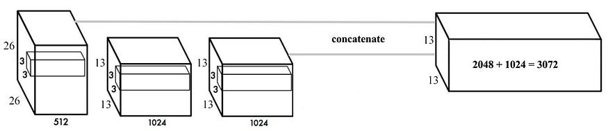
Instead of running region proposal networks at various feature maps to many resolutions, like in Faster R-CNN and SSD (Single-Shot Detector), the modified YOLO version adds a passthrough layer which brings features from an earlier layer at 26 x 26 resolution.
This layer concatenates the higher-resolution features with the low-resolution ones by stacking adjacent features into different channels, turning the
26 x 26 x 512 feature map into a 13 x 13 x 2048 one, which is again concatenated with the original 13 x 13 x 1024 features.
✅ This expanded feature map, having a feature map of 13 x 13 x 3072, provides access to fine-grained features, and improves the YOLO model
by 1%.

7. Multi-Scale Training
YOLO originally used an input resolution of 448 x 448, which got changed to 416 x 416 by adding anchor boxes. But as the modified network has no FC layers (just convolutional and pooling layers), it can be resized on the fly.
The network is modified every few iterations — every 10 batches, it randomly chooses a new image dimension size. As the model downsamples by a factor of 32, the network learns the following resolutions, {320 x 320, 352 x 352,… 608 x 608}.
The fact that the same network can predict detections at various resolutions means we can now fine-tune the sizes for speed and accuracy.
At low resolutions, YOLOv2 is a fairly good and accurate detector ideal for smaller GPUs, high framerate video or multiple video streams.
At 288 x 288, it runs at 91 FPS and gives 69.0 mAP, comparable in accuracy to Fast R-CNN (70.0 mAP), but much better than the latter in speed (Fast R-CNN has a speed of just 0.5 FPS) [scores for VOC 2007]At high resolutions, YOLOv2 is a state-of-the-art detector giving 78.6 mAP on the VOC2007 dataset, it’s accuracy the highest among the models compared in the paper, while still having a real-time speed of 40 FPS.


Further Experiments
On the VOC 2012 detection dataset, YOLOv2 obtains 73.4 mAP, better than the original YOLO, Fast R-CNN, Faster R-CNN, and SSD 300.
This performance is comparable to ones by SSD512 (74.9 mAP) and ResNet (73.8 mAP), but YOLOv2 is the fastest (2–10 times) among them all.

On the COCO 2015 test-dev dataset, using the VOC metric, IOU = 0.5, YOLOv2 gets 44.0 mAP, comparable to the performances of SSD512 and Faster R-CNN.

To summarize, the table below lists the design decisions which mostly led to increases in mAP in YOLOv2, compared to YOLO, except two — using a fully convolutional network with anchor boxes & using the new network (Darknet19, we’ll look at this shortly).
The anchor box approach increased recall from 81% to 88%, but decreased the mAP from 69.5 to 69.2, while the new network reduced computation by 33%.

Phew! That were a lot of changes made just to make the model better, next let’s take a peek at how YOLOv2 is faster than YOLO.
Faster than YOLO
VGG-16 is the classification feature extractor used by most detection architectures (source); though it gives state-of-the-art performance, it’s unnecessarily complex (it uses ~31 billion floating point operations for a single pass over a single image at 224 x 224, thus requiring heavy computing power).
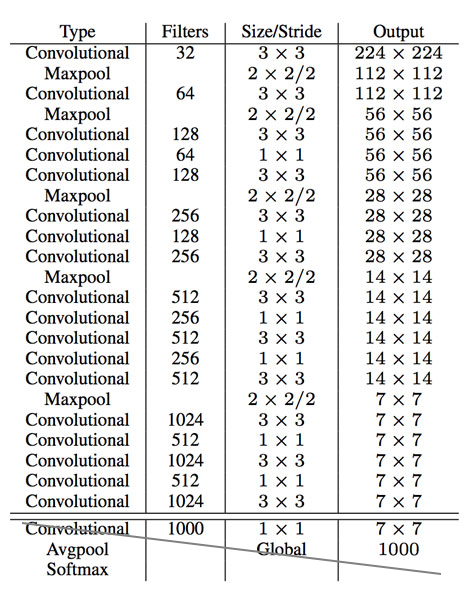
Based on the Googlenet architecture, YOLOv2 uses a custom framework named Darknet19 (it has 19 convolutional layers, 5 max pooling layers).
✅It is better than VGG-16 because —
- It requires just 5.58 billion f.p. operations compared to ~31 billion in VGG-16, so it’s much faster
- Though it uses relatively low f.p. operations, it still scores a higher top-5 accuracy, getting 91.2% on ImageNet, compared to 90% by VGG-16 (YOLO used 8.52 billion f.p. operations and got a top-5 accuracy of 88%)
- They used the then-novel global average pooling to make predictions, compared to max pooling layers in VGG-16
- Batch normalization was used for stabilizing training and model regularization, it also made convergence faster
- 1 x 1 convolutional filters were used between 3 x 3 layers to compress the features (source)

Global average pooling layers are used to cut down overfitting by reducing the number of parameters in the network.
It’s a type of dimensionality reduction where tensors having dimensions of
(h x w x d) are converted to have a dimension of (1 x 1 x d)

Given below is the model structure of Darknet19.

The portion striked through in the image above is replaced with three 3 x 3 conv layers (1024 filters each) followed by a 1 x 1 conv layer with the number of outputs needed for detection, the final output is 7 x 7 x 125.

The YOLOv2 paper explains in depth, the hyperparameters (and their values) the authors used for best performance. I won’t go into that detail and bore you, but just know it’s all out there if you’re interested.
Stronger than YOLO
Finally, let’s look at the new features in YOLOv2 and YOLO9000 which make them better than their previous counterpart.
One feature specific to object detection datasets when compared to image classification datasets is that, the former have limited labeled examples. Vanilla detection datasets contain images in the range 10³-10⁵ with dozens to hundreds of tags. (e.g. the COCO dataset has 330K images with just 80 object categories)
Classification datasets are huge in that, they contain millions of images with thousands to tens of thousands of classes (e.g. ImageNet contains around 14 million images with ~22,000 distinct object classes).
Because labeling images for detection (predicting bounding boxes, performing non-maximal suppression, etc.) is expensive compared to labeling images for classification (simple tagging), detection datasets are difficult to scale to the level of classification datasets.
What if we could combine the two types of datasets together and build our network such that it could perform both classification and detection, & even better, detect objects in images which have classes that it hasn’t seen any labeled detection data for?
Hierarchical Classification — combining detection and classification datasets
Turns out, the paper presented a solution to the very same question we posed above.
We can combine images from both types of datasets during training, but we have a problem — while detection datasets have simple object labels like “bottle”, “microwave” and “bus”, classification datasets are more diverse and detailed in their classes (I spotted 15 different kinds of snakes here on a cursory glance, like “boa constrictor”, “ringneck snake”, and “green mamba”). So how do we merge labels from both datasets?

Typically, we’d use softmax classification but it’s not an option here because the classes are not mutually exclusive. What I mean is, softmax only works when no class is related to each other, thus we can easily have the probability of an object belonging to a class, and all probabilities will
add to 1.
In our case, “tarantula”, “garden spider” and “wolf spider” are related to each other, as an example.

Instead, we can start from scratch, forgetting all the knowledge we have about the labels being related to each other.
ImageNet labels are extracted from WordNet, an online lexical database that structures concepts and how they relate to each other.
Structured as a directed graph, different object classes can belong to the same parent class (hyponym), which can then be among various types of objects, etc.
For example, in WordNet, “laughing owl” and “great grey owl” are both hyponyms of “owl”, which is a type of “bird”, which is a type of “mammal”, etc.
To build the tree, we follow these steps —
- Observe the visual nouns in ImageNet and follow their paths through the WordNet graph to the root node (“physical object”)
- Because many synsets just have a single path, we add all of them to our tree
- For the concepts left, we iteratively examine them and add those paths that grow the tree by as little as possible (if a concept has 2 paths to the root, one having 5 edges and the other having 3 edges, we’ll choose the latter)

We thus obtain the WordTree, a hierarchical model of visual concepts.
Instead of performing a softmax on 1000 classes (of ImageNet), the WordTree will have 1000 leaf nodes corresponding to the original labels plus 369 nodes for their parent classes.
At every node, we predict the probability of each hyponym of a synset given that synset.
Say I want to find the probability of the node “terrier”.
For this, we’ll predict the following probabilities (probability of a Norfolk terrier given that the object is a terrier and so on)
Pr(Norfolk terrier | terrier)
Pr(Airedale terrier | terrier)
Pr(Sealyham terrier | terrier)
Pr(Lakeland terrier | terrier)
...
If we’d like to compute the absolute probability for some node, we follow the path through the tree to the root node and take a product of all conditional probabilities.
The follow example is for computing the probability that a picture is of an Airedale terrier.
Pr(Airedale terrier) = Pr(Airedale terrier | terrier)
                     * Pr(terrier | hunting dog)
                     * ....
                     * Pr(mammal | animal)
                     * Pr(animal | physical object)
We always assume that the picture contains an object, so Pr(physical object) = 1.

For computing the conditional probabilities, Darknet19 predicts a vector of 1369 values and the softmax over all synsets that are hyponyms of the same concept is calculated.

As you can see, all hyponyms of the synset “body” (head, hair, vein, mouth, etc.) come under one softmax calculation.
Thanks to WordNet, DarkNet19 achieves 90.4% top-5 accuracy on ImageNet, keeping all the parameters same as before.
Following is a representative image, showing how classes from ImageNet and COCO datasets are merged using the WordNet structure.

YOLO9000 — Simultaneous Classification and Detection
Now we have a technique to combine object detection and image classification datasets together to get one huge datasets, and the best part is, we can train our model to perform both classification and detection.
Using the technique above, we combine the COCO dataset (for detection) and the top 9000 classes from the full ImageNet dataset (for classification) — the combined dataset contains 9418 classes.
You might observe that the size of ImageNet is very huge compared to COCO, it has multiple orders of magnitude higher number of images and classes.
To tackle this unbalanced dataset problem, we oversample COCO so that the ratio of images in ImageNet and COCO is 4:1
On this dataset we train our YOLO9000 model, using the architecture of YOLOv2 but 3 anchor boxes instead of 5 to limit the output size.
On a detection image, the network backpropagates loss as usual — objectness (box confidence score, i.e. confidence that the image contains an object), bounding box, and classification error

On a classification image, the network backpropagates objectness loss and classification loss.
For objectness loss, we backpropagate using the assumption that the predicted box overlaps the ground truth label by ≥ 0.3 IOU.
For classification loss, we find the bounding box that predicts the highest probability for the class and the loss on just its predicted tree is computed.

YOLO9000 is evaluated on the ImageNet detection task, which has 200 fully labeled categories.
44 of these 200 categories are there in COCO as well, so the model is expected to do better on classification than detection (because it has lots of classification data thanks to ImageNet, but relatively less detection data).
Though it hasn’t seen any labeled detection data for the remaining 156 disjoint classes, YOLO9000 still gets 19.7 mAP overall, 16.0 mAP on those 156 classes.
This performance is better than the one by DPM (Detectable Parts Models, which use a sliding-window approach to detection), but then YOLO9000 is trained on a combined dataset having both classification and detection images, & it is simultaneously detecting 9000+ object categories.
All in real time.

On ImageNet, YOLO9000 does well in detecting animals but performs poorly when it comes to learning classes such as clothing and equipment.
This can be attributed to the fact that COCO has lots of labeled data for animals, thus YOLO9000 generalizes well from the animals there; but COCO has no bounding box labels for objects such as “swimming trunks”, “rubber eraser”, etc. so our model doesn’t do well on such categories.

Kudos to you if you read till here. Now you are aware of how YOLOv2 and YOLO9000 are better, faster and stronger than the original YOLO model.
We saw how we can combine object detection and image classification datasets using WordNet (hierarchical classification) and get great performance. Using this technique, YOLO9000 can detect over 9000 object categories, and simultaneously perform classification and detection, that too in real time!
Using multi-scale training (training the model on images of different resolutions), we saw how we can make the YOLOv2 model more robust and make training more stable.
In future articles, we’ll see how we can implement YOLOv2 ourselves using the Darknet library, and talk about even better versions of YOLO, like YOLOv3 and v4.
Hope this article enlightened you about the YOLOv2 and YOLO9000 architectures.
Follow me on LinkedIn and Medium for upcoming articles :)
References
- BatchNorm (TDS article), (research paper)
- Network in Network research paper
- Global Average Pooling
- COCO Dataset (80 classes)
- WordNet — An online lexical database
- YOLO9000 slides
- Anchor boxes in Faster R-CNN research paper (Section 3.1.1)
- Object detection with YOLO, YOLOv2 and YOLOv3 (TDS article)
- 1000 classes of ImageNet
- WordNet owl example
- WordNet terrier example
- ImageNet detection task
