Diabetic Retinopathy Detection

Published in

Analytics Vidhya

23 min readOct 15, 2020

Rapid Screening and Early diagnosis of Disease Retinopathy using Scanned Retinal images and underlying Deep Learning models.

https://static01.nyt.com/images/2019/03/10/business/10aieyedoctor1/10aidoctor1-facebookJumbo.jpg

We have seen the advancement of deep learning in solving complex business problems in Banking, E-commerce, and Autonomous Transportation. But have you ever imagine that an AI model can diagnose a disease without a doctor? Yes! It’s actually happening in Sankara Eye Hospital, Bengaluru. Let’s get dive deep into solving this case study using Deep Learning.

Introduction:

What is Diabetic Retinopathy?

Diabetic retinopathy is the most common form of diabetic eye disease and usually affects people who have diabetes for a significant number of years. The risk of diabetic eye is for aged people especially working persons in rural and slum areas.

It increases with age as well as with less well-controlled blood sugar and blood pressure level and occurs when the damaged blood vessels leak blood and other fluids into your retina, causing swelling and blurry vision. The blood vessels can become blocked, scar tissue can develop, and retinal detachment can eventually occur.

**Difference Between Normal retina and Diabetic Retina**

Retinopathy can affect all diabetics and becomes particularly dangerous by increasing the risk of blindness if it is left untreated. The condition is easiest to treat in the early stages, which is why it is important to undergo routine eye exams before it becomes too late for treatment.

Problem Statement:

Technicians of Aravind Eye Hospital have collected a large number of scanned retinal images of diabetic persons by traveling through rural areas and hosted the problem in Kaggle as a competition where the best solutions will be spread to other ophthalmologists through APTOS.

They want us to build a system where it takes the retinal image of a patient and tells us the severity of diabetic retinopathy.

Why we need an automation system?

We have scanned images, then why can’t we use trained doctors to diagnosis the disease instead of using the black box system? Is there a need for automation here? Yes!, There are a couple of advantages here like below.

It helps the patient especially to those who can’t afford a doctor.
It reduces human efforts especially when the number of doctors is less.
Useful for people in rural areas where medical screening is difficult to conduct.
It saves the time involved in diagnosing a disease.

Table of contents:

Chapter-1: Data Extraction / Importing the Data and Setup

Chapter-2: Exploratory Data Analysis

Step_2–1: Analysis of Dataset.
Step_2–2: Data Exploration.
Step_2–3: Image Pre-Processing.

Chapter-3 : Evaluation Metrics

Step_3–1: Transforming Output Variables.
Step_3–2: Cohen kappa metric.

Chapter-4: A solution through Deep Learning - Concept of Convolutional Neural Networks

Step_4–1: Training Baseline models.
Step_4–2: Data Augmentation.
Step_4–3: Transfer Learning.

Chapter-5: Ensembles

Chapter-6: Model Interpretability - Working on the Black box model.

Step_6–1: Introduction to Grad-Cams.
Step_6–2: Error Analysis.

Chapter-7: Conclusions

Chapter-1 : Data Extraction / Importing the Data and Setup:

I am using Google Colaboratory to get access to high RAM (12 GB), 50 GB hard drive space, and GPU for faster training. Know more about colab notebooks here.

Source Of Data:

I have extracted the data from the Kaggle under APTOS 2019 Blindness Detection competition. You can directly download the data from here.

It will take around 36 minutes for downloading the data on a normal local machine. I am using Curlwget (chrome extension) for faster downloading. To know more about this follow this link.

It will give aptos2019-blindness-detection.zip file in 2–3 minutes. However, we can extract all the below files by unzipping that file using the following command in 4–5 minutes

unzipping the file

The competition has given 5 files occupying 9.52 GB of space.

i. test_images: directory containing test images (total 1928 files).

ii. train_images: directory containing training images (total 3662 files).

iii. sample_submission.csv: Format of submission file to the competition(28.26 KB).

iv. test.csv: the path to test images as id_code (24.48 KB).

v. train.csv: the path to training images as id_code along with target class labels as diagnosis (53.66 KB).

Chapter-2 : Exploratory Data Analysis:

Step_2–1: Analysis of Dataset:

Observations:

Both the train and test datasets are not too large.
The training dataset is three times larger than the test dataset.
Risk of overfitting on model training.
Need for Transfer learning and data augmentation.

The clinicians have rated each image for the severity of diabetic retinopathy on a scale of 0 to 4. It is a multi-class problem with 5 target classes

**Severity level of Diabetic Retinopathy**. Reference link here.

Observations:

Dataset is heavily imbalanced
There are 10 times more images with No DR condition than the images with Severe condition.
Need for adding class weights
0 - No DR, 1 - Mild, 2 - Moderate 3 - Severe, 4 - Proliferative DR

Image Analysis:

Collecting the height and width of all images in training data

There is no standard shape for images in both training and test images.
We need to bring all the images into a standard resolution which should be relatively high else the informative pixels will get compressed.

Splitting the Dataset:

After splitting the data we need to store the files permanently so that there will be no problem of data leakage in future training.

Step_2–2: Data Exploration:

Each row depicts the severity level of the disease retinopathy.
There are four major problems in our dataset which will make our model difficult to spot the identities.

Images with dark color Illumination: Some of the images are very dark which will mislead our model towards incorrect classification.

Images with different color inversion: Here some images are completely different in color shades like blue, pink, and green.

Images with uninformative extra dark black pixels: This is the major issue because while resizing the image most of the informative pixels will become small.

Images with irregular cropping: There are four different patterns of cropping in the dataset.

Most of the training images are type-I and type-III, test images with type-III.

Step_2–3: Image Pre-Processing:

Steps involved in Image Preprocessing:

All the images contain a black background. And we can observe some of the images have extra dark pixels at the sides of the images. So in step-1 involves cropping of those extra dark pixels.
We can see that there is no fixed size for image width and image height. Hence we do resize of an image in step-2.
A lot of images are shrunk and some images have a circular shape and some are cropped at edges. Hence in step-3, we are drawing a circle from the center to give a similar shape to all the images.
As we can observe most of the images are taken in different resolutions. Where some are taken in lighting conditions and some in dark. we are adding a smoothing technique to remove the noise in images by using a gaussian blur to the images. This gives our final preprocessed image.

After applying image preprocessing on training dataset:

**Plotting sample Images of each class Before and After Preprocessing**

Image to vector conversion:

image 2 vector conversion

Image preprocessing is a time taking process. Hence I am storing preprocessed images into a vector so that there will be no need of running the above code every time running the program.

Loading processed data

Everything is perfect. Now we are ready for model training :)

Chapter-3 : Evaluation Metrics:

Step_3–1: Transforming Output Variables:

There are five outcomes in our model i.e., [0,1,2,3,4]. Now we can transform these labels either using

One hot encoding: It refers to splitting the column which contains numerical categorical data into many columns depending on the number of categories present in that column. Each column contains “0” or “1” corresponding to which column it has been placed.

For example, if the target label is 2 then it will be encoded as [0,0,1,0,0]

Ordinal Regression: It is used to learn ranking or ordering on instances, which has the property of both classification and metric regression. The learning task of ordinal regression is to assign data points into a set of finite ordered categories i.e., A teacher rates students performance using A, B, C, D, and E (A>B>C>D>E)

For example, if the target label is 2 then it will be encoded as [1,1,1,0,0] which means the sample with class-2 also belongs to the classes before it (0,1)

According to this paper using ordinal regression especially in the case of categorical target variables that are ordered that too in healthcare will be of more help.

Ordinal Regression

Step_3–2: Cohen kappa metric:

The competition has given a weighted kappa score as an evaluation metric. Let’s just see what it is meant for.

It is used to measure the degree of agreement between raters among categorical data.
It is a simple extension to accuracy where it finds the simple percent agreement calculation (True predictions / Total predictions) while the kappa score makes it more robust by considering the agreement that occurred by chance.

Cohen’s kappa metric. Reference link here.

Quadratic Weighted Cohen’s kappa score:

The weighted kappa allows disagreements to be weighted differently and it is useful when scores are ordered.
It makes use of three matrices:

The matrix of observed scores.
The matrix of expected scores.
Weight matrix

Quadratic Weighted Cohen kappa score. Reference link here.

Why using a weighted kappa metric?

There are a lot of metrics to compare the results like confusion matrix, accuracy, recall, precision, etc.., Then why to use a new metric?

It is useful when the target labels are ordered like [0,1,2,3,4].
In case of disagreement, the score is given according to the distance of predicted and observed elements. It is not only taking care of agreement but posing penalty on the disagreement.
The score will be higher if the true prediction is 3 and the model predicted as 2 and will be lower if the model prediction is 4. This property will be very helpful because in medical getting higher than expected will be okay because on later diagnosis it can be rectified. But if the patient got class-1 and it is predicted as class-0 then it will be a problem because that patient is ignored which can adversely affect the patient as well as the reputation of the hospital.

Read more about the kappa score here and here.

Calculating kappa metric

Chapter-4 : A solution through Deep Learning — Concept of Convolutional Neural Networks

Step_4–1: Training Baseline models:

Computing Class Weight:

Since the data set is highly imbalanced adding class weight can make it balanced by adding weights to each of the classes.
The class with more weight means they are less in samples. Similarly, the class with less weight means they are more in samples.

Custom Callbacks:

Here we will modify the callback class in TensorFlow in order to print the kappa metric on each epoch on validation data.

Custom callback for printing validation kappa score on each epoch

Model Training:

Convolutional Neural Networks(CNN):

Machine Learning research has focused extensively on object detection problems over time. But various things make it hard to recognize objects like segmentation, lighting, Deformation, etc..,

Convolutional Neural Networks can be used for all work related to object recognition from hand-written digits to 3D objects. The real value of CNN came out in the competition of ILSVRC-2012 competition on the ImageNet-a dataset with approximately 1.2 million high-resolution training images. The winner of the competition, Alex Krizhevsky (NIPS 2012), developed a very deep convolutional neural net of the type pioneered by Yann LeCun. These have made them so popular.

First I started with a baseline model to estimate the final score and to make necessary changes in model training. Here I used simple

3 Convolutional layers with a fixed kernel size of 2x2 and padding = the same with Relu activation.
2 Max pooling layers with a fixed kernel size of 2x2.
Global Average Pooling layer after max pooling
One dropout layer
4 Dense layers

Implementation of the Baseline model

After running the model for 30 epochs I got a kappa_score of 0.6931 which is relatively good to start with.

Performance Metrics on Validation dataset:

**Performance metrics of the baseline model**

We can see that there are a lot of miss classifications in class-2.
Most of the samples from class-1 and class-4 are predicting as class-2.
Also, there are no correct predictions on class-4 at all. This means the model enables us to draw meaningful patterns in differentiating class-4 samples.

Now let’s try model training with Alexnet architecture.

**AlexNet Architecture**. Reference link here.

Highlights of the paper:

Using Relu activation instead of Tanh to add non-linearity.
Local Response Normalization.
Overlapping Pooling.
Dropouts.
Training on Multiple GPU’s with
1. Model Parallelism
2. Data Parallelism

Implementation of AlexNet architecture

After running the model for 30 epochs I got a kappa score of 0.7758 on validation data which is better than the baseline model.

Performance Metrics on Validation dataset:

**Performance metrics of Alexnet model**

Here also most of the samples from class-1, class-3 are predicting as class-2.
It started making a good number of predictions on class-1 and class-4.
This model training is far better to differentiate between classes than baseline model training.

Step_4–2: Data Augmentation:

We hardly have ~3k images on training and ~500 images for validation. Any deep learning model with a small dataset will prone to overfit easily which is not there in baseline and alexnet but still, it’s good to have a large set of data.

By augmentation, we can increase the size of our dataset at runtime without actually storing them in our system. I used the following four augmentation techniques which will increase our dataset by 4 times.

Horizontal flipping
Vertical flipping
Rotation range
Zoom range

Read more techniques of augmentation here.

Data augmentation

**Images generated after augmentation of one sample**

Step_4–3: Transfer Learning:

Transfer learning focuses on storing knowledge gained while solving one problem and applying it to a different but related problem.

I am using pre-trained models that are trained on the imagenet dataset.

How it is useful in model training ?:

Imagine you want to solve task A but don’t have enough data to train a deep neural. Exactly matches our case.
Knowledge gained while learning to recognize one problem(cars) could apply when trying to recognize another problem (trucks).
For better results. These models are trained on a large set of images and able to extract meaningful features in differentiating one set of classes among others.

All the pretrained model architectures are extended with the following three layers.

GlobalAveragePooling2D:
From the last convolutional layer of any pretrained model which generates as many feature maps as the number of target classes, and applies global average pooling to each in order to convert each feature map into one value by taking the average of it.
Dropout
Dropout works by randomly setting the outgoing edges of hidden units to 0 at each update of the training phase. Which will be used as a sort of regularization in order to avoid overfitting during model training.
Dense
This layer contains 5 units each represents the individual class with sigmoid activation.
Optimizer: Adam
loss: binary cross-entropy
metric: accuracy and weighted kappa

Implementing Global average pooling 2D, dropout and dense layers

Visual Geometry Group (VGG):

VGG has 16 or 19 layers starting with simple 3x3 filters in the first convolutional layer.
The number of channels increased with terms of 2 and Nh, Nw decreased with a factor of 2.
Though it contains lots of parameters, the model is simple with fixed 3x3 filters and stride=1 and the same padding in convolutional layers.
2x2 filters with stride=2 in max-pooling layers.

VGG16 Architecture

Tensorboard Visualization:

We can see that there is no much major difference between training and validation. Hence we can say that our model is not overfitted.

After training the model for 30 epochs I got a kappa score of 0.8931 on validation data.

Performance Metrics on Validation dataset:

VGG19 Architecture

Tensorboard Visualization:

We can see that there is no much major difference between training and validation. Hence we can say that our model is not overfitted.

After training the model for 30 epochs I got a kappa score of 0.9128 on validation data.

Performance Metrics on Validation dataset:

DenseNet Architecture:

DenseNet was developed specifically to improve the declined accuracy caused by the vanishing gradient in high-level neural networks.
Due to the longer path between the input and output layer, the information vanishes before reaching its destination.
It is a 5-layer dense block with a growth rate of k = 4.
An output of the previous layer acts as an input of the second layer by using composite function operation. This composite operation consists of the convolution layer, pooling layer, batch normalization, and non-linear activation layer.

DenseNet with 121 layers:

=> 5+(6+12+24+16)*2 = 121

5 — Convolutional and Pooling layer
3 — Transition layers(6,12,24)
1 — Classification layer(16)
2 — Dense Block(1x1 and 3x3 Conv)

DenseNet Architecture

Tensorboard Visualization:

We can see that there is no much major difference between training and validation. Hence we can say that our model is not overfitted.

After training the model for 30 epochs I got a kappa score of 0.923 on validation data.

Performance Metrics on Validation dataset:

Model is making good number of predictions over all classes.

Residual Networks:

Instead of directly stacking a few layers to fit an underlying H(x) mapping. Explicitly let these layers to fit a residual mapping F(x).
Now,
F(x) = H(x) — x
H(x) = F(x) + x

Now this residual mapping(F(x)+x) is called skip connections which skips one or more layers.
These connections perform identity mapping and their outputs are added to the outputs of the stacked layers.
These connections add neither extra parameters nor computational complexity.

**ResNet-50 Architecture**. Reference link here.

Resnet Architecture

Tensorboard Visualization:

We can see that there is no much major difference between training and validation. Hence we can say that our model is not overfitted.

After training the model for 30 epochs I got a kappa score of 0.9091 on validation data.

Performance Metrics on Validation dataset:

ResNet-152 Architecture

Tensorboard Visualization:

We can see that there is no much major difference between training and validation. Hence we can say that our model is not overfitted.

After training the model for 30 epochs I got a kappa score of 0.9146 on validation data.

Performance Metrics on Validation dataset:

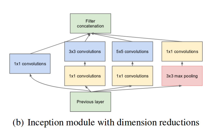
Inception Networks:

The inception model allows us to apply multiple filters(1x1, 3x3, 5x5) and even max-pooling layer on the same level and concatenate the results. Thus the network essentially would get a bit ‘wider’ rather than ‘deeper’.

Inception v3 Architecture.

Tensorboard Visualization:

We can see that there is no much major difference between training and validation. Hence we can say that our model is not overfitted.

After training the model for 30 epochs I got a kappa score of 0.9014 on validation data.

Performance Metrics on Validation dataset:

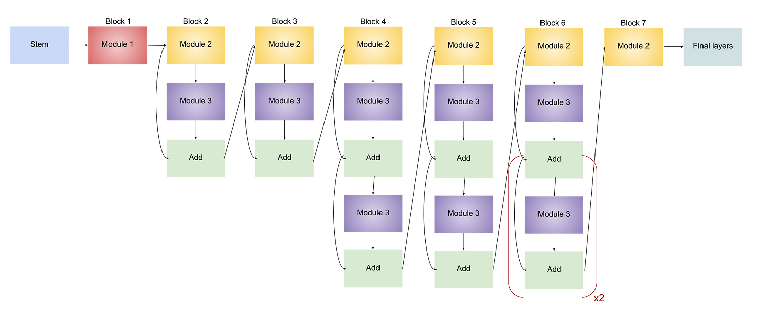
Efficient Net Networks:

It starts with the stem.

Stem Architecture

Generally, the models are made too wide, deep, or with a very high resolution. Increasing these characteristics helps the model initially but it quickly saturates and the model made just has more parameters and is therefore not efficient. In EfficientNet, they are scaled in a more principled way i.e. gradually everything is increased.
The architecture consists of 7 blocks. These blocks further have a varying number of sub-blocks whose number is increased.
Finally ends with Final layers.

Step_6–1: Introduction to Grad-Cams:

Step-1: Takes an image and passes it to a model and takes the gradients with respect to each feature at a particular convolutional layer(mostly last convolutional layer) also by making use of the predicted class labels.
Step-2: Resizing the gradients to the size of the image.
Step3: Plotting the heat map of that gradients to know the activations in predicting that class label with respect to the input image.

Where the cyan color indicates the higher activations in predicting the class (ball here).

Step_6–2: Error Analysis:

Error rate = False predictions on that class / total predictions on that class

Analysis of false predictions on each class

class-0 has an error rate of 2.05
class-1 has an error rate of 27.84
class-2 has an error rate of 24.92
class-3 has an error rate of 34.72
class-4 has an error rate of 28.47

Count of Predictions which are less than the true predictions:

Here 10 samples actually belong to class-1 but predicted as class-0. These 10 cases are the most important to examine because these patients actually have retinopathy(mild stage) but are predicted as having No retinopathy.

Plotting those 10 Samples:

Chapter-7 : Conclusions:

The final solution to our problem statement:

After applying a couple of pretrained models, Ensembling those models has given a top score of 0.9314.
But here our goal is not only to give the best score but to provide a system that makes a prediction with an explanation.
Here I have chosen DenseNet which has given the next best score of 0.923 val kappa score for model interpretability and ensemble of all pretrained models for final model prediction.

About Model Training:

Encoding class labels using ordinal regression.
Adding class weight to balance the dataset.
Binary cross entropy as loss function with Adam optimizer.
Used Densenet architecture which is pretrained on the imagenet dataset. After running the model for 30 epochs, the model has given a score of 0.923 on the validation dataset which will be taken for model interpretability
Ensembling for final model prediction.

Overall Observations of the case study:

We can see their is high rate of misclassification among class-2 an class-3.
More sample data on training can improve the performance on these classes.
More preprocessing and with different sigmax (low than the actual) can be useful in predictions.
Their is high chance of data shrinkage on square crop images. Hence we need to come up with different approach (manual cropping is best).
Drawing circle on the images has made all the samples to be equal and also helped in interpretation of model predictions. Partially Resolved the problem of over expose and under expose.
Ensembles has worked best in our case. But it loses the property of interpretability.
Advanced pretrained models on complex datasets especially trained on medical(eye) can fairly improve our model.
Need to come up with differet augmentaion techniques to increase the size of the data set.

Future Work:

Deep learning is the task of experimenting with multiple parameters. Hence I want to hyperparameter with more possible values.
Using different augmentation techniques to increase the size of the dataset.
Making use of 2015 data(the similar problem of binary classification) in Kaggle.
Want to make a web API so that every ophthalmologist can access my work.
I want to experiment by adding more convolutional layers in each model architecture.
Making use of Super-resolution GANS to increase the resolution of images.

References:

As an aspirant of becoming a Data Scientist brings me here. This includes my final work for this case study. Thank you for reading my article.

You can also read to my other articles and case studies here.

You can check the .ipynb for a full code snippet of this case study in my Github repository.

Follow me for more such articles and implementations on different real-world case studies in data science! You can also connect with me through LinkedIn and Github

I hope you have learned something out of this. There is no end for learning in this area so Happy learning!! The signing of bye :)

Diabetic Retinopathy Detection

Step_2–1: Analysis of Dataset:

Step_2–2: Data Exploration:

Step_2–3: Image Pre-Processing:

Step_3–1: Transforming Output Variables:

Step_3–2: Cohen kappa metric:

Step_4–1: Training Baseline models:

Computing Class Weight:

Model Training:

Step_4–2: Data Augmentation:

Step_4–3: Transfer Learning:

Step_6–1: Introduction to Grad-Cams:

Step_6–2: Error Analysis:

Overall Observations of the case study:

Written by Chaitanyanarava