Exploring Other Face Detection Approaches(Part 2) — SSH
In these series of articles, we are exploring various other approaches of detecting faces rather than the common ones. In the previous article (Part 1), we discussed about RetinaFace.
In this part we’ll discuss about SSH: Single Stage Headless Face Detector.
We will be covering four different types for face detection architectures:
1. RetinaFace
2. SSH: Single Stage Headless Face Detector
3. PCN: Progressive Calibration Network
4. Tiny Face Detector

SSH: Single Stage Headless Face Detector
Most CNN based detector, whether detecting objects or only faces, converts classification network into two stage detection systems. In the first stage convolutional layers proposes a set of bounding boxes for the object and then the remaining layers of classification network referred as ‘head’ are used to classify the proposals. The head of the classification network can be computationally very expensive and had to be performed for every proposed bounding box.
Here comes the role of SSH as it is headless i.e it doesn’t require any fully connected layers to perform the classification of proposals but rather can perform both the detection and classification in a single stage by only using convolutions thus reducing the inference time. SSH is also scale invariant by design. Instead of relying on external multi-scale pyramid as input for detecting faces of various scales, it detect faces from various depths of the network.
Architecture

Here, I am splitting the overall architecture into 3parts for better understanding.
1. Detection Module, which detects the faces.
2. Context Module, part of detection module.
3. Training and loss function.
- Detection Module
As you can see it a fully convolutional network followed by 3 detection modules (M1, M2 and M3) on top of feature maps with stride 8, 16 and 32. The detection module consists of binary classifier and regresser for detecting and localizing faces.
To solve the localization problem, they defined the anchor set in dense overlapping sliding window fashion. At each sliding window location, K anchors are defined which has the same center as that of window and different scales but considering only those anchors whose aspect ratio is 1, to reduce the amount of anchors. If the feature map connected to Mi has size
(Wi x Hi), then there would be (Wi x Hi x Ki) anchors with aspect ratio 1 and scales {S¹,S², … }

It includes a context module[discuss below] for effective receptive field. The number of output channel, X is set to 128 for M1 and 256 for M2 and M3.
At each convolutional layer in Mi, the classifier decides whether the anchor contains the face or not. A 1x1 conv layer with 2xK output channels acts as classifier for face/not face and another 1x! conv layer with 4xK output channels regresses the bounding box.
Al the 3 detection modules have 3 different strides which helps in detecting small, medium and large faces respectively {Making it scale invariant}. All the convolutional layers defined in overall architecture are from VGG-16 network. For M1, to reduce the memory consumption number of channels are reduced from 512 to 128 and feature map fusion is done by summing up the upsampled conv5-3 feature with conv 4-3 feature. For large face detection M3 has a max pooling layer of stride 2.
2. Context Module

As anchors are getting classified and regressed in convolutional manner in detection module, using a larger convolutional filter will resemble like increasing the window size around proposal in 2-stage detector. Modeling the context in this way will increase the receptive field proportional to the stride of corresponding layer resulting in target scale in each detection module.
5x5 and 7x7 filters are used for convolutional in context module but to reduce the number of parameters it is being deployed using 3x3 filters.
3. Training and Loss Function
The network has three multi-task losses for each of the detection module. To specialize each module for different range of scales, back-propagation is done only for those anchors who are assigned to face in their specific range.
This is implemented by distributing anchors based on their size to three detection modules {smallest anchors are assigned to M1, then to M2 and M3}. An anchor is assigned to ground-truth face if its IoU is higher than 0.5.
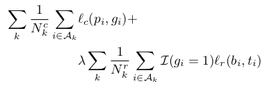
Here, the first part of the loss function is cross entropy loss for face classification. the indec k denotes the number of detection module in the network and A_k defines the set of anchors in M_k detection module. Predicted and ground truth label is pi and gi respectively.
As discussed above anchor is assigned to ground-truth bounding box if its IoU is greater than 0.5 and similarly negative labels are assigned to anchor is its IoU is less than 0.3 with any ground-truth bounding box. This combination of anchors forms ((N_k)^c) in module M_k which takes part in classification loss.
The second part of the loss function is smooth l1 bounding box regression loss. pi represents the predicted four bounding box values[x,y,w,h] and ti is the assigned ground-truth regression target for the i’th anchor in module Mk. I(.) is the indicator function that limits the regression loss only to positive anchors. ((N_k)^r) becomes the number of anchors in module M_k which takes part in regression loss.
Lastly, OHEM is used for training the SSH. It is applied in each detection module separately i.e for each Mk, we select negative anchors with the highest score and positive anchors with the lowest score with respect to the weights of the network in that iteration, to create mini-batch. 25% of the mini-batch is reserverd for the postive anchors as negative anchors are more in numbers.
At the time of inference, the predicted boxes from different scales are joined together using NMS to get the final output.
Conclusion
We learned about a new face detector which is a fast and lightweight face detector that, unlike two-stage proposal/classification approaches, detects faces in a single stage.