The journey of Gradient Descent — From Local to Global
In my previous article, I covered the intuition of gradient descent with the implementation of the mathematics behind it to reach the minimum value of cost function. It seemed as easy as walking down the hill (Yeah that’s what gradient descent is).
The last article was wound up with the line: sometimes, it may happen that instead of reaching global minima, the value of cost function gets stuck at the local minima or the saddle point.
Also I would like to show you something which may ruin your enthusiasm you had.
In Deep Learning, there are different types of cost function which have a different shape other than this. Thus this simple shape of cost function does not exist while dealing with different cost functions.

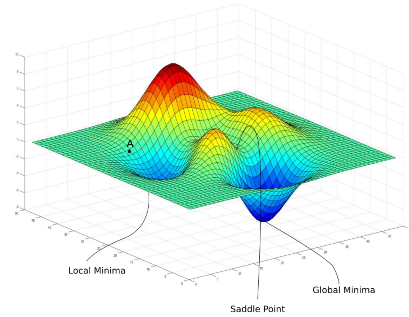
Instead, it is mostly with many convex surfaces, thus it looks somewhat like this :

So as shown, The Cost function actually has a lot of local minima and we need to get to the global minima.
So let’s begin.
While training, it is important for the cost function to reach the minimum value, which is the global minima (lowest values of the cost function) to give nearly accurate results. But, we may risk falling into a local minima (the lowest of all the nearby values) or the saddle point. Since it is not the real minimum value, the results may not come up to expectations.


We cannot totally avoid getting stuck at local minima or the saddle point, but still, we can use several techniques in order to help mitigate this problem.
Stochastic Gradient Descent (SGD) and Mini-Batch SGD
SGD and Mini-Batch SGD are the transformed version of Gradient Descent(GD). Consider a dataset with n examples (n>10⁶). In GD, we consider all the n points for reducing the cost function which makes this algorithm use a high computation power. Whereas in SGD, only a single (n=1) data-point is used in each epoch and the parameters are updated accordingly. In Mini-Batch SGD, we take k data-points (k<n) from the sample and update our parameters. These methods of selecting the samples less than n make the algorithm computation friendly.
In gradient descent, the value of the cost function decreases gradually, which increases the chance of meeting local minima and makes it impossible to get out of that point. Whereas in SGD, the variation is abrupt. Thus it reduces the probability of getting stuck at local minima, and even if it gets stuck, chances are that it will definitely come out due to its jolting movement.

Regularization
When the cost-function reaches local minima, the process of updating parameters tries to come to a conclusion, but we need to prevent this situation. In that case, we penalize the large weights. At the local minima even if the derivative is zero, then also the weights keep updating due to the regularizer added. There are two types of regularizers L1(Lasso) and L2(Ridge).
L2 Regularization (Ridge)
The equation of the cost function in L2 regularization is :

L1 Regularization (Lasso)
The equation of the cost function in L1 regularization is :

Here, When the derivation of J(Y’, Y) will be zero at local minima, the regularizer term will penalize the cost function, and hence the parameters will get updated even if they are at local minima, and at global minima, the updation will not take place, thus we can avoid getting stuck in local minima using Regularization.
Momentum
Momentum simply adds a fraction of previously updated weights to the current weight.
We can write the weight updating equation as follows :

Here β is the momentum factor and it ranges between 0 and 1 (both not inclusive) it is again a hyperparameter that can be tuned.
I found a good visualization of momentum on YouTube by Diego Inácio, Do watch it.
Altering the Learning Rate — α
Instead of using a constant learning rate throughout the training process, we can use Learning Rate with constantly changing values with time.
The equation of altering learning rate can be represented in the simple form

Here, T and α_o are hyperparameters that can be tuned. Here t can vary from 0 to T and hence α has an inverse relationship with t. Here α changes until t hits T, during this time, the model is said to be in a searching phase, Thus, the learning rate decreases with time, and hence movement along the error surface can be made smoother.
Winding-up
Here we saw that Standard Gradient Descent can be optimized in a way such that we can solve the issue of getting stuck at the local minima using various techniques, each technique adds up a hyperparameter for us to tune. However, there are many algorithms like Adam, Adagrad, and Adadelta which tend to work much faster, but also are more difficult to implement.
Here is an illustration of the converging speed of different algorithms.

Here we come to an end.
See you in the next story.
Thanks.
