Phishing URL Detection Using ML

Phishing stands for a fraudulent process, where an attacker tries to obtain sensitive information from the victim. Usually, these kinds of attacks are done via emails, text messages, or websites. Phishing websites, which are nowadays in a considerable rise, have the same look as legitimate sites. However, their back-end is designed to collect sensitive information that is inputted by the victim. Discovering and detecting phishing websites has recently also gained the machine learning community’s attention, which has built the models and performed classifications of phishing websites.

This could be done using different methods like one is visual similarity of the web page, another is using text vectorization technique, using logo, using URLs etc. In this case study we are going to learn about the different techniques and also how machine learning helps to achieve our objective.

Business problem:

Phishing is a big problem in the cybersecurity domain. An attacker does this by different techniques such as by creating or replicating a page similar to a legitimate page so that the user can mistakenly give personal information or account information to the attacker, another is by email like lottery winning or any product at 95% discount etc in which attackers try to get user account information on transaction completion etc. That’s why hacks like two factor authentication come into picture.

In this domain by creating a web application in which the user feeds the URL and the application returns if the URL is legitimate or not we derive a machine learning approach. As there are websites available for this like PhishTank but these websites depend on users’ vote, but by extracting the features from urls and using machine learning models we can achieve something similar by also providing the probability score.

Business constraints:

• Low latency required.
• Errors can be very costly as if the user performs a transaction on a phishing site, it may cost the user money or information loss.
• Probabilistic interpretation is desirable.

ML formulation of the business problem:

Binary Classification Problem

1 -> Phishing

0 -> Legitimate

Performance Metrics:

roc_auc_score

• As the ROC which stands for receiver operating characteristic is a plot used to illustrates the performance of binary classification problem using a variying threshold where the False positive rate is x-axis and True positive rate is y-axis.
• The roc_auc_score is a scoring function that computes the area under the ROC and summarized it in single number.
• It calculate based on predict_proba which gives the probability of the respective predicted values.

Data Collection:

The phishing urls are collected using the link: https://www.phishtank.com/developer_info.php

It consists of 12841 urls.

The legitimate urls are collected using the link: https://hackertarget.com/top-million-site-list-download/

It consists of 1000000 urls.

Sampled the urls at random and took 10000 urls from it.

Features are extracted from the urls using FeatureExtractor.ipynb which consist of several functions and are sub categorized into three as follows:

• Url based features
• DNS Records based features
• Page Content/ html based features

To extract the features, there were requirements to send HTTP requests and do the rest of scraping using bs4 and domain fetching things using whois database so created a class named as requests_fetcher where by using multi-threading capabilities of it, parallelizing or speeding up the requests. This is the main class which then inherited and method get_response of it is overridden according to the feature extraction processes.

# https://stackoverflow.com/a/68583332/5994461
class requests_fetcher:
  THREAD_POOL = 1024

  # This is how to create a reusable connection pool with python requests.
  session = requests.Session()
  session.mount(
      'https://',
      requests.adapters.HTTPAdapter(pool_maxsize=THREAD_POOL,
                                    max_retries=3,
                                    pool_block=True)
  )

  def get_response(self, url, verify = False):
    try:
      self.response = self.session.get(url, timeout = 2, verify = verify)
      # logging.info("request was completed in %s seconds [%s]", response.elapsed.total_seconds(), response.url)
      # if response.status_code != 200:
      #     logging.error("request failed, error code %s [%s]", response.status_code, response.url)
      if 500 <= self.response.status_code < 600:
          # server is overloaded? give it a break
          time.sleep(5)

      return self.response

    except:
      self.response = ""
      return self.response

  def download(self, urls, cl = None):
      with ThreadPoolExecutor(max_workers= self.THREAD_POOL) as executor:
          # wrap in a list() to wait for all requests to complete
          if(cl):
            ls = list(executor.map(cl.get_response, urls))
          else:
            ls = list(executor.map(self.get_response, urls))
          return ls// explanation of the above function

Top five rows of final feature extracted csv file

This dataset contains 22932 rows/samples and 27 columns/features.

Existing Approaches:

1. Blacklist/ whitelist: by putting the legitimate urls in the whitelist or the phishing urls in the blacklist.
2. Machine learning based CANTINA: It uses the most repeated words on the page to check the page in a search engine. Let say, by using tf-idf of words in the whole HTML page, using the frequency and sorting the words accordingly, it selects the top 5 words and use them as page descriptor for the search in search engine and if the domain name comes within top N search results it states that the url is legitimate else phishing.
3. CANTINA+ : In this apart from what is engineered in CANTINA, 15 new features extracted from the HTML page are also used in the dataset.

Drawback: The technique works well but there are some limitations with this as it requires additional searching operation which creates additional network load. Another is if the attacker promotes the url to the top searches, the system may fail to predict if the url is legitimate or phishing.

Approach taken to solve this problem:

This is started with feature extraction that helps to determine the nature of url followed by data preprocessing like handling missing values, removing constant features, removing outliers etc. Then comes exploratory data analysis to know more about the features, their importance, relation with the target value. After which comes the feature engineering which later helped the model to find out the patterns more accurately. Then comes the feature scaling and modeling.

Exploratory Data Analysis

Split the dataset into train and test set to avoid data leakage i.e. only train dataset should be present in model training as an information not the whole dataset, to avoid variance. If during model training the whole dataset involves, it predicts well for that dataset but not for the new queries comes during production.

Data types and missing values

X_train.info()
<class 'pandas.core.frame.DataFrame'>
Int64Index: 18345 entries, 11992 to 18551
Data columns (total 27 columns):
 #   Column                      Non-Null Count  Dtype  
---  ------                      --------------  -----  
 0   url                         18345 non-null  object 
 1   url_having_IP_Address       18345 non-null  int64  
 2   url_having_at_symbol        18345 non-null  int64  
 3   url_length                  18345 non-null  int64  
 4   url_depth                   18345 non-null  int64  
 5   url_redirection             18345 non-null  int64  
 6   url_http_domain             18345 non-null  int64  
 7   url_sortining_service       18345 non-null  int64  
 8   url_prefix_suffix           18345 non-null  int64  
 9   url_standard_port           18345 non-null  int64  
 10  url_google_index            18345 non-null  int64  
 11  dns_record                  18345 non-null  int64  
 12  domain_age                  18345 non-null  int64  
 13  domain_registration_length  18345 non-null  int64  
 14  statistical_report          16161 non-null  float64
 15  page_mouse_over             18345 non-null  int64  
 16  page_right_click_disable    18345 non-null  int64  
 17  page_pop_up                 18344 non-null  float64
 18  page_iframe                 18343 non-null  float64
 19  page_website_forwarding     18342 non-null  float64
 20  link_pointing_to_the_page   18323 non-null  float64
 21  submit_email                18321 non-null  float64
 22  redirection_count           18315 non-null  float64
 23  server_from_handler         18345 non-null  int64  
 24  page_favicon                11586 non-null  float64
 25  ssl_state                   18345 non-null  int64  
 26  result                      18345 non-null  int64  
dtypes: float64(8), int64(18), object(1)
memory usage: 3.9+ MB

Insights:

This dataset is having null values in 8 columns:

statistical_report, page_pop_up, page_iframe, page_website_forwarding link_pointing_to_the_page, submit_email, redirection_count and page_favicon.

Column url is textual data.

Column result is our target feature.

Constant features

Those features that contains only one value for all the observations, they donot provide any information in classifying the task so its better to remove such bad features

# dropping constant urls
X_train = X_train.loc[:,X_train.apply(pd.Series.nunique) != 1]

Handling missing values

# https://github.com/ResidentMario/missingno
import missingno as msno
# Gives positional information of the missing values
msno.matrix(X_train.drop(columns = ['url', 'result']))
<matplotlib.axes._subplots.AxesSubplot at 0x7f8e5dd46b10>

msno.dendrogram(X_train.drop(columns = ['url', 'result']))
<matplotlib.axes._subplots.AxesSubplot at 0x7f8e554428d0>

# percentage of data missing in features wrt. total no. of rows
 
missing_variables = X_train.isnull().mean()[X_train.isnull().mean() != 0]
missing_variables
statistical_report           0.119052
page_pop_up                  0.000055
page_iframe                  0.000109
page_website_forwarding      0.000164
link_pointing_to_the_page    0.001199
submit_email                 0.001308
redirection_count            0.001635
page_favicon                 0.368438
dtype: float64

To deal with null values there are many techniques like :

dropping the null values,

replacing it with mean/mode/median

imputing with most_frequent/ new category

creating a new feature for the missing values

using model based imputer etc.

We must know what could be the reason of it to avoid bias using statistical tools like : MCAR, MAR, MNAR. link

Missing completely at random: This comes where there is no systematic differences between the missing value and the target ones.

Missing at random: When the missingness is not random but rely on some other independent feature.

Missing at not random: It happens when the missingness it causes by choice, the variable is thus related to the variable itself.

Missing valued feature => statistical_report

missing_statistical_report['result'] = X_train.result

missing_statistical_report.groupby('statistical_report')['result'].mean()
statistical_report
0    0.455797
1    0.453205
Name: result, dtype: float64

There is no relation between the missingness of this feature and the dependent value, concluding it as Missing completely at random type.

# creating an unknown variable as -1

X_train['statistical_report'] = X_train['statistical_report'].fillna(-1)

Missing valued feature => page_favicon

missing_page_favicon['result'] = X_train.result

missing_page_favicon.groupby('page_favicon')['result'].mean()
page_favicon
0    0.456293
1    0.454089
Name: result, dtype: float64

This is Missing completely at random type. As the missing values are 36% rows of the total dataset so its better to create a new column than to drop it.

X_train['page_favicon'] = X_train['page_favicon'].fillna(-1)

Missing valued feature => redirection_count

missing_redirection_count['result'] = X_train.result

missing_redirection_count.groupby('redirection_count')['result'].mean()
redirection_count
0    0.455351
1    0.545455
Name: result, dtype: float64
# filling na with 1    
X_train['redirection_count'] = X_train['redirection_count'].fillna(1)

Dropped the less frequent null valued rows.

Uni-variate Feature analysis : Used to analyze single independent feature at a time, wrt. dependent feature.

print('Unique values in result column: ',X_train.result.value_counts())

sns.countplot(X_train.result)
Unique values in result column:  1    10333
0     7988
Name: result, dtype: int64

% of phishing data points:  56.39975983843677
% of legitimate data points:  43.60024016156323

The result feature is having values 0 for legitimate data points and 1 for the phishing data points.

There is slightly unbalanced dataset.

url based features

url_length and url_depth are numerical features whereas others are categorical features and numerically formatted as 0 and 1.

url_length

The distribution of url_length is highly positive skewed. There are a very few points bent towards the right side means few data points are having larger url length.

The above figure represents the url length is having outliers.

Detected and removed outlier using quantiles, which tends to dropped %age of points from the dataset: 9.513672834452267

In this figure, conclude that the length of phishing points per density is larger than the legitimate points as the dentity is almost equal but on figure the density of legitimate is more on mode as compared to the phishing points. Its a helpful feature to distinguish between the classes.

url_depth

The above figure represnts the url length is having outliers for the result value 1 i.e. phishing.

Detected and removed outlier using quantiles, which tends to dropped %age of points from the dataset: 10.278682591386175

In this figure, conclude that the length of phishing points is larger than the legitimate points. Its a helpful feature to distinguish between the classes.

url_having_at_symbol

This plot is showing that there all legitimate points belongs to value 0 for this feature. And the phishing points are in both 0 and 1 value. But still there is an overlap for the value 0.

url_redirection

This plot shown above states that there is an overlap for the value 1 of this feature wrt. the target values.

There are only 4 points having value 0 for this feature and all of them belongs to class 0 i.e. legitimate.

This is not a useful feature.

url_http_domain

The plot shown above that for all the data points that are legitimate, this feature value is 0 and for the phishing it is 1 for most of the points.

This is a useful feature.

url_sortining_service

url_prefix_suffix

The plots states that these features are not so useful as for both the values which are quite distinguishable inspite of which the target is almost overlapping.

url_standard_port

url_google_index

This plot shown above states:

url_standard_port is a bad feature as almost all the points belongs to value 1 and the target is highly overlapped.

url_google_index is a good feature, the target is easily distinguishable.

domain based features

Both are useful features. As for the feature name domain_age, the result 0 i.e. legitimate is heavily belongs to value 0 of this feature. And for dns_record there are more frequecy of phishing points for the value 1.

page based features

Both the features plotted above are not helpful ones as they are overlapping for both the 0s and 1's.

redirection_count feature makes no sense of any distinguishabilty for the result. submit_email could be helpful as very less phising points are having value 0 for this as compare to legitimate ones.

server_from_handler and ssl_state are bad features. In page_favicon feature, -1 denotes unknown value but is high in case of legitimate, it could be hellpful feature.

PCA

Its a technique used to reduce the dimentionality of dataset.

It uses the covariance matrix of the data using which able to fetch the eigen vectors of it which are the principal components.

link

This plot gives intuition that only 15 components or features are giving 95%+ explained variability.

Feature selection

Its a preprocessing step in machine learning. It selects the important features by maximizing the relevant information using score functions and helps to discover the redundant and irrelevant features so to avoid them during the model training process.

Mutual information

It compute scores based on the intersection between two random variables where the random variables are independent and dependent ones. And it is similar to the information gain.

I(X ; Y) = H(X) — H(X | Y)

Where I(X ; Y) is the mutual information for X and Y, H(X) is the entropy for X and H(X | Y) is the conditional entropy for X given Y.

def select_features(X_train, y_train):
  '''
  This function takes X and y as input
  calculates K best features using scoring function, for this mutual_info_classif is being used as score function
  returns the k best features with their scores
  '''
  fs = SelectKBest(score_func=mutual_info_classif, k='all')
  fs.fit(X_train, y_train)
  return fs

Using above plot we can conclude that the top 5 Weak features:

1. url_sortining_service
2. link_pointing_to_the_page
3. page_pop_up
4. page_right_click_disable
5. statistical_report

As the dataset is small, its better not to delete any feature to avoid overfitting.

Correlation matrix

It is used to find the linear relationship between the variables.

Its coefficients are categorized as positive, negative and zero.

Using above plot the few insights are as follows:

1. url_length, url_depth, url_http_domain, url_google_index, domain_age having strong correlation with result.
2. There is multi-collinearity in dataset. Could be helpful in feature engineering, by constructing new features and perform further feature interaction.

Feature engineering

Created a few new features as follows:

• length_depth = url_length + url_depth
• port_redirection = url_standard_port + redirection_count
• var_median = df.median(axis = 1)
• var_max = df.max(axis = 1)
• var_std = df.std(axis = 1)
• var_sum = df.sum(axis = 1)

Model training

The process of inputting the data to an Machine learning algorithm so it could be trained in a manner to identify the patterns from the dataset.

First cut approach:

I tried with generalized spot classification modeling approach, it is like autoML where the train dataset gets involved in model training process and model is not definite, traction the same dataset in multiple models to find out which model performs well in comparison to other using cross_val_score and score function.

The models included in this are as follows:

LogisticRegression

• As name implied, it uses logistic function to model a binary classification problem.

• It is a linear model.
• It take several assumptions into consideration which include absence of multi-collinearity, the observations are independent,etc.
• Performing feature scaling before modeling is useful as its a distance based algorithm.

Support Vector Machine Classifier

• It is a linear model based classifier which can solve linear and non linear problems based on right kernel.

• It works based on margin maximization i.e. separation of two classes of data points by increasing the margin space.
• It works well where the number of columns is greater than the number of rows but not works well with large dataset due to its train time complexity.

DecisionTreeClassifier

• It is a tree based classifier creates the model by building a decision tree. Each node of which specifies an feature and each branch descending from that node specifies one of the possible values for that feature.

• It does not require feature scaling.
• It selects the nodes based on information gain, gini impurity and entropy.
• It is advantageous where interpret-ability is required but is unstable i.e. small change in the data can lead to a large change in its structure.

KNearestNeighborsClassifier

• It is an instance based model i.e. it doesn’t learn anything in training, it uses distance based similarity to select k nearest points for the query point thus predicts the points having majority.

• As it is a distance based algorithm, it requires features to be scaled. It suffers from curse of dimentionality.
• It doesn’t work well with large dataset due to its time complexity.

GaussianNB

• Its a classification technique based on Bayes theorem having an assumption of feature independence.
• It handles both continuous and categorical data and can handle large datasets.

# prepare models
models = []
models.append(('LR', LogisticRegression()))
models.append(('KNN', KNeighborsClassifier()))
models.append(('Decision Tree', DecisionTreeClassifier()))
models.append(('NB', GaussianNB()))
models.append(('SVM', SGDClassifier(loss = 'hinge')))

# evaluate each model in turn
results = []
names = []
scoring = 'accuracy'
for name, model in models:
	kfold = model_selection.KFold(n_splits=5)
	cv_results = model_selection.cross_val_score(model, X_train, y_train, cv=kfold, scoring=scoring)
	results.append(cv_results)
	names.append(name)
	msg = "%s: %f (%f)" % (name, cv_results.mean(), cv_results.std())
	print(msg)
Output
LR: 0.994823 (0.002677)
KNN: 0.926516 (0.005201)
Decision Tree: 0.959527 (0.003563)
NB: 0.893640 (0.005924)
SVM: 0.906282 (0.041549)

Using above approach we can conclude that the logistic regression is the one which performs very well both in terms of speed and accuracy.

Hyper parameter tuning

The process of finding the best parameters for parametric model so it performs well.

Using GridSearchCV for this, which loops through all combinations of the parameters passed in the form of dict object and thus evaluates the model for each and every combinations using cross validation method by taking the score function as a scoring parameter.

logistic regression

Feature Scaling

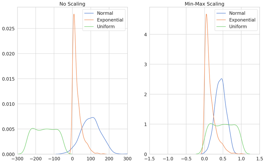
To normalize the range of features, they are scaled. It is essential in cases where distance is used to calculate the similarity between the data points.

Here, MinMaxScaler is used which re-scaled the range of features to scale the range between 0 and 1 or -1 and 1 by giving the feature_range as a parameter.

ls=[10**-4, 10**-2, 10**0, 10**2, 10**4]
tuned_parameters = [{'logisticregression__C': ls}]

# creating pipeline
pipe = make_pipeline(MinMaxScaler(), LogisticRegression())
#Using GridSearchCV
search = GridSearchCV(pipe, tuned_parameters, scoring = 'roc_auc', cv=5, return_train_score= True, n_jobs =-1)
search.fit(X_train, y_train)
Output:
Best hyper parameter:  {'logisticregression__C': 10000}
Model Score:  0.9826442776350583
Model estimator:  Pipeline(steps=[('minmaxscaler', MinMaxScaler()),
                ('logisticregression', LogisticRegression(C=10000))])

Confusion matrix for Logistic Regression Model

In this plot, the false negatives or type 2 error is 14% of the total negative data-points. Still, the true positive and true negatives are good which states that we can trust this model.

Applying Ensembles

Ensemble methods is a machine learning technique that combines several base models where the base models may be the same or different in order to produce one optimal predictive model which is combined set of final predictions.

Random Forest Classifier

• It is an ensemble based model where the decision tree is used as its base learners.
• The collection of decision trees used bootstrap sampling for random features selection and model training then aggregated and returns the prediction based on voting scheme thus known as bagging i.e. bootstrap aggregation.

• It is interpret-able and returns feature importance based on the aggregate FI of base learners using information gain or so.
• The base learners i.e. decision tree should be modeled in a manner to gain high variance which later on aggregation gets balanced. Thus as in decision tree, most of the hyper parameters are same in random forest as well like, max_depth, n_estimators, min_samples_split, min_samples_leaf etc.

depth = [1, 10, 50, 100, 500, 1000]
n_estimators = [100, 200, 300, 400, 500]
tuned_parameters = [{'randomforestclassifier__max_depth':depth, 'randomforestclassifier__n_estimators': n_estimators}]

# Applying RandomizedSearchCV with k folds = 5 and taking 'roc_auc' as score metric
pipe = make_pipeline(MinMaxScaler(), RandomForestClassifier())
clf = GridSearchCV(pipe, tuned_parameters, scoring = 'roc_auc', cv=5, return_train_score= True, verbose = 10, n_jobs= -1)
clf.fit(X_train, y_train)
Output:
Best hyper parameter:  {'randomforestclassifier__max_depth': 500, 'randomforestclassifier__n_estimators': 500}
Model Score:  0.9937430027759891
Model estimator:  Pipeline(steps=[('minmaxscaler', MinMaxScaler()),
                ('randomforestclassifier',
                 RandomForestClassifier(max_depth=500, n_estimators=500))])

Confusion matrix of RF Classifier

This confusion matrix showing that the true positives and true negatives are comparatively higher as compared to the false positive and negative so we can trust this model. The precision and recall thus the f1 would be higher too because of high true values.

Feature Importance

importance = rf_model.steps[1][1].feature_importances_

plot_feature_importance(importance, X_train.columns,'RANDOM FOREST')

According to this plot, apart from url_http_domain and url_depth, the features constructed in feature engineering are quite helpful.

Model Comparison

+---------------------+---------------------------------+-------+-------+---------------+
|        Model        |         Hyper parameter         | Train |  Test | roc_auc_score |
+---------------------+---------------------------------+-------+-------+---------------+
| Logistic regression |             C=10000             | 0.975 |  0.97 |     0.968     |
|    Random Forest    | max_depth=500, n_estimators=500 | 0.995 | 0.987 |     0.995     |
+---------------------+---------------------------------+-------+-------+---------------+

Looking at this plot, its easily identifiable that the random forest classifier is the winner.

Future Work:

We can try with a transformer based approach by splitting each URLs into single character tokens and appending a classification token “CLS” at the end. Applying that tokenized input to padding using another token as “PAD” and so on. It may drastically improve the performance but for this we need the dataset to be more sophisticated in terms of quantity and quality.

References:

• https://www.appliedaicourse.com/
• https://arxiv.org/pdf/2009.11116v1.pdf
• https://www.sciencedirect.com/science/article/pii/S2352340920313202
• https://arxiv.org/ftp/arxiv/papers/2110/2110.13424.pdf
• https://www.phishtank.com/
• https://www.alexa.com/topsites
• https://github.com/ResidentMario/missingno
• https://scikit-learn.org/stable/modules/generated/sklearn.feature_selection.mutual_info_classif.html
• https://machinelearningmastery.com/feature-selection-with-categorical-data/
• https://machinelearningmastery.com/compare-machine-learning-algorithms-python-scikit-learn/

Github Repo:

GitHub - joshiKuldeep/Phishing-Detection-using-ML