The world through the eyes of CNN.
Convolutional Neural Networks is a class of deep learning models widely used in the field of computer vision & its applications. Convolutional Neural Networks are highly proficient in the task of identifying objects, recognising faces in a crowd & they even form the basic building block of self-driving cars. Given a bunch of training images, CNN can learn to identify the objects in the image by analyzing its features. As the image propagates forward from one layer to the next, CNN learns to pick up more complex features & patterns.

When we train a Convolutional Neural Network, does it exactly comprehend the image as we humans do?
It becomes difficult to answer this question if we perceive deep learning models as a black-box, we feed in data/image to the model & the model outputs its prediction. Even though the prediction may be accurate, The model isn’t truly intelligent if it doesn't perceive images like how we humans do. After all, we are trying the recreate human intelligence on a computer or Artificial Intelligence.
It becomes easier for us humans to debug a deep learning network if we understand the flow inside the network rather than interpreting it as a black box.
How does the image look at each layer?
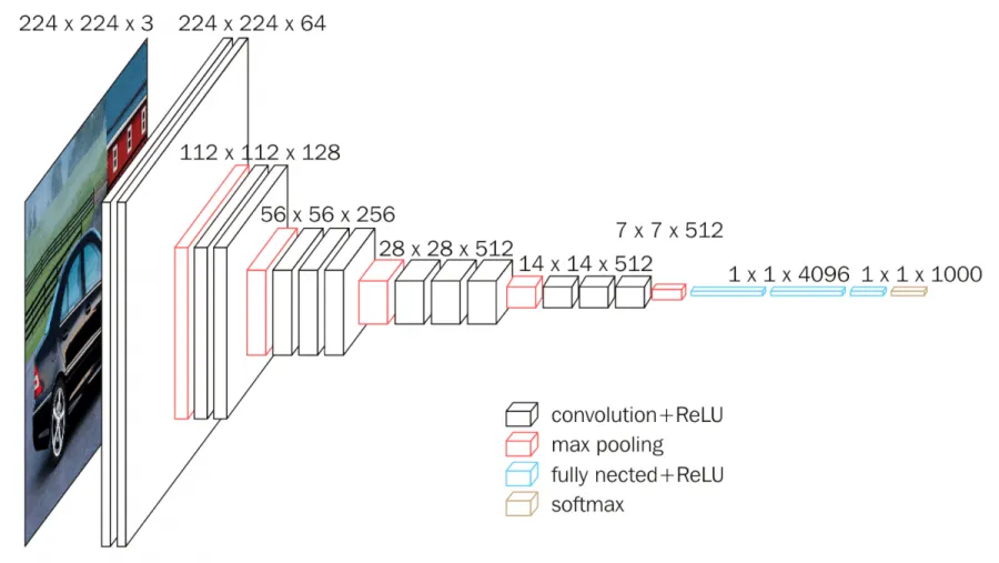
By visualizing the feature/activation map of a filter at a particular layer after the convolution operation gives us insight on “what the network is looking at each stage of the convolutional neural network”. Let us consider a CNN model known as VGG16 which has achieved benchmark results on ImageNet classification. Using this network will provide us with great insight into how the network visualizes the objects in images.
The filters at the first few initial layers extract direction & colour, these primitive(edges & colour) feature maps get combined into basic grids, textures & patterns. These, in turn, get combined to extract increasingly complex features which resemble parts of objects. As we move down the network the features extracted become more complex to interpret.

The above diagram shows feature maps at different stages on the network. The feature maps at the initial(lower) layers encode edges & direction i.e. horizontal or vertical lines, the feature maps obtained at the middle of the network visualize textures & patterns, the feature maps at top layers depict parts of objects & objects in the image. Let’s visualize this image of tesla car at different stages of VGG16.

Low-level/Primitive features
The lower level feature maps extract edges & lines of the images. These are primitive feature extractors (filters) which pick up minor details of the image like lines , curves & dots.
The output feature maps are from the initial layers of VGG16 network trained on ImageNet dataset. The primitive features horizontal, vertical & 45⁰ lines help depict the shape of the car’s body.


Mid-Level features
Primitive feature maps combine to produce simple shapes such as circles, squares, ellipse etc. The mid-layer features provide more information than the first, for example, the filters learn to detect corners, replicate basic patterns, textures & shapes.
The mid-level features resemble the circular shape of the tyre, the door, bumper etc. We can generalize that mid-level features depict textures, patterns in images.


Higher-Level features
Higher-level features depict complex patterns which resemble parts of objects in images which tend to be a unique trait of for that class(object), which contributes to classification score for that class as well. The feature maps below depict the face of a dog, eyes etc.


As we go deeper, CNN produces complex patterns like eyes, nose etc. The above feature maps depict different parts of a dog, its nose, eyes, furr, floppy ears, tail many more.
The feature maps of tesla at higher levels of VGG16 are as shown below. The images might be difficult to comprehend, but by looking closer at the image on the right we notice details such as the windows, the tires etc.


Look at the flamingo feature map, it represents the flamingo bird from different perspectives, similarly with the billboard table. These are features or patterns unique to that particular class of image.
Thus, the feature maps at higher levels of the network help in distinguishing two objects by presenting features which remain unique to a particular object. The CNN can then easily classify the input image to its corresponding class.
These visualizations of a trained CNN model not only gives us insight into its operations which was previously considered as a black-box but also aids in diagnosing the network & rectifying the network architecture to improve its performance.
Although, looking at trippy patterns which CNN's visualize don’t precisely pinpoint what’s making the CNN classify an image to a particular class. The visuals at higher layers form complex patterns which are not understood by humans. If we could visualize, the exact region/part on the input image a feature/activation map is looking, this can be done by projecting the feature maps back on the input image which would highlight the region on the image CNN is looking at through that layer & its corresponding filter (aka heatmap).
Diagnosing Convolutional Neural Networks.
Why is it important to visualize feature maps of CNN?

In this image from hackevolve, the football region of the image is highlighted which is a great indication that the network is looking at precise features to classify the object as football. The image on the right is the Gradcam output of the network at a particular filter. You can think of it as a heatmap, the highlight being the region of interest. The highlight shows that the network has learnt the pentagon-hexagon pattern found on a football & uses this specific trait to classify.
By visualizing it makes easy for us to understand where the network is looking & helps deduce if the network is cheating.
How can a Convolutional Neural Network cheat?
Imagine if the network was looking at the green grass to classify the object as football and not the ball itself. The highlighted region is the grass & not the ball.
The network can then misclassify a basketball on a football pitch as a football. Meaning the network is not looking close enough or at relevant features.
Here are a few more examples of how a network can cheat.
- A Convolutional Neural Network associating birds with blue sky can classify an aeroplane as a bird if an image of an aeroplane in the sky is shown to the network. Vice-versa also works.
- The network looking at the plants/trees while classifying the image as an elephant. The network fails to capture the trunk, its ear, the tusk or any features specific to an elephant.
Techniques to make CNN more transparent.
To clearly understand where the CNN is looking at by visualising the region of interest on the input image (visualising heatmaps) provides us with a deeper understanding of the network’s working by making it more transparent. By analysing these heatmaps one can make changes to the network, add or remove few layers, hyperparameter tuning, add more images to the dataset or apply a different strategy of data augmentation.
Class Activation Maps aka CAM
One of the techniques for visualizing which parts of the image the CNN is looking at while classifying. The visualization is a heatmap highlighting the “class-specific regions on the image”.
The idea proposed by CAM requires CNN to have a specific architecture which it can take advantage of. CAM requires a global average pooling layer at the penultimate layer (last but one), I.e. GAP layer before fully-connected layers.

Input image passes through the CNN layers extracting features at each layer. The layer before GAP will have n feature maps which is the result of all the features captured by all the preceding layers. n can be any value that is specified by the network, each of those n feature maps is of width u & height v. In in the above image, the red, blue, green feature maps indicate the final feature maps before GAP.
What is Global Average Pooling?
Global average pooling turns the feature map into a single number by taking an average of the pixel values. If there are n feature maps, GAP results in n single-valued tensors.

Global average pooling makes the network invariant to spatial translations or perturbation of an image.
Fully connected layers & the classification score.

After GAP the network outputs n single value numbers which get converted into classification scores. The classification score for the class “Australian terrier” is given as,
Y^australian-terrier = w1 x n1 + w2 x n2 + …. + wn x n. (Here n is the GAP output).
How to obtain the Class Activation Map.
Instead of multiplying the weights associated with Australian-terrier with the GAP output, we multiply the weights with the feature maps before GAP.
Assume, we had n feature maps f1, f2, f3 … fn of width u & height v, before global average pooling. The weights associated with Australian-terrier neuron are w1, w2, w3 … wn.
CAM^aus = f1 x w1 + f2 x w2 + f3 x w3 + … + fn x wn.

The resultant feature map is of width u & height v (same as f1,f2,…,fn). The Class Activation Map dimensions are the same as the feature map dimensions (A1, A2, A3 … An.)
The Classification Activation Map is upsampled to match the input image dimensions & overlayed on top to see results.


The output class activation map is the summation of all the feature maps. In the above, we have n feature maps, each of which looks at different parts or patterns on the dog, one feature map focuses on its legs, while the other on its Furr & coat, while another on its face. The heat map region is enclosed of all its individual feature map.
Here, is another example of the network picking up on different traits of a palace such as its trademark dome, renaissance styled architecture etc. The network predicts a high probability to the class castle, without disregarding church, altar or monastery cause they all look the same.
Limitations of Class Activation Maps.
- The Convolutional Neural Network needs to be modified, it doesn't have a Global Average Pooling layer.
- Addition of GAP layer requires re-training of the network.
- Visualizations or heatmaps can be obtained with respect to the last CNN layer.
GradCAM: Gradient-based Class Activation Map
To address the limitations of faced by class activation map, gradient-based class activation maps were introduced. Rather than directly associating the weights of the prediction layer with the feature maps, GradCAM computes the gradient of the output score with respect to the feature maps of a convolutional layer.
By computing the gradient (derivative) of the classification-score with respect to the individual feature maps, we obtain a value which indicates how much of the feature-map is being contributed to the classification score. i.e. the rate at which the classification score changes wrt changes in the feature map.
For example, we compute the classification score of class dog wrt one of its feature maps which visualizes the floppy ears in dogs. If the floppy ears are more prominent in the feature maps than they were, the classification score would increase, if they were less prominent, the classification score might decrease. By computing the gradient we obtain a contribution metric of a feature map towards classification.

Here, y^c is the output classification score of class c (before softmax) & A^k is the kth feature map of a convolution layer i & output of filter j from layer i. GradCAM computes the gradient(derivative) with respect all features 0 …. k. The output can be called as a gradient-feature map.

After computing k gradient-feature maps, we perform global average pooling on each of the k gradient-feature maps.
The resultant output global average pooled gradient feature maps (alpha-k), we perform a weighted linear combination of ak & feature maps of the convolutional layer.

Each feature map is multiplied with its own global average pooled gradient feature map (alpha-k with feature map A^k). This weighted linear combination results in a coarse heatmap of the same size as the feature map A^k. We apply ReLU to the coarse heatmap as we are only interested in features of the image which have a positive influence on its prediction.


How does GradCAM overcome the limitations of CAM?
- One can compute the gradient of output classification score with respect to feature maps of any convolutional layer, unlike CAM where the last layer feature maps can only be used.
- The network doesn’t need any modification, GradCAM can be computed without Global Average Layer in the network. (Note, we perform GAP operation of the gradients which is not a part of the network).
Here are the GradCAM outputs from different parts of VGG16 network trained on ImageNet dataset.


Conclusion
The implementation of the concepts can be found in this notebook.