Understanding And Implementing Neural Style Transfer
Neural style transfer is a artistic method of combining style and content of two seperate images into a single image using Deep learning methods.
Pre-requisites: Basic understanding of CNN’s and Keras.


So what is Neural Style Transfer (NST) ???
According to Wikipedia,
Neural Style Transfer refers to a class of software algorithms that manipulate digital images, or videos, to adopt the appearance or visual style of another image.
The NST algorithm which we are going to study is based on the paper A Neural Algorithm of Artistic Style by Leon A. Gatys et.al . NST algorithms provide an artificial system based on Deep Neural Network that creates artistic images of high percptual quality.
Creation of artistic kind of images is a branch of computer vision called non-photorealistic rendering but these methods involve direct manipulation of image pixels rather than on feature space of an image.
As we deal with feature space of an image we make use of Convolution Neural Networks(here we use VGG-19 architecture) which are already trained on huge datasets like Imagenet(1000 classes) for object detection task.
Why do we make use of CNN in NST??

- CNN’s are class of Deep Neural Network which are powerful in image processing tasks. Each layer of a CNN produce a feature maps of an input image which are filtered versions of input images.
- We can use the feature maps of each layer to reconstruct the input image. The feature maps are the multi layer representation of an image which are produced as an output by the layers of CNN.
- CNN’s help in capturing the representation of images in feature space rather than in pixel space.
- The higher layers of CNN’s capture the global information of an image rather than pixel representations. The global representation capture the high level content of an image. In contrast the lower level layers capture the exact pixel values of the original image. So we use feature responses from higher layers for “content representation”. Here we use feature maps of “conv5_1” layer of VGG-19 which is top most convolution layer.
- The “style representation” of an image is obtained by building a multi-scale feature space. This feature space contains correlations between the different filter responses of multiple layers. Here we will use the feature maps of “conv1_1”, “conv2_1”, “conv3_1”, “conv4_1”, “conv5_1” in a cummulative way.
By including the feature correlations of multiple layers, we obtain a stationary, multi-scale representation of the input image, which captures its texture information but not the global arrangement.
Implementation of NST
The process involved in implementing this algorithm :
- Select two images where one of them is style reference image and another is content base/target image. We will get better results if the chosen style reference image has more texture and patterns.
from keras.preprocessing.image import load_img, img_to_array
target_image_path = 'img/portrait.jpg'
style_reference_image_path = 'img/transfer_style_reference.jpg'
width, height = load_img(target_image_path).size
img_height = 400
img_width = int(width * img_height / height)
2. Select a network (here we use VGG19) which is already trained on some dataset for some specific tasks like object detection. The reason we are using already trained network is that they already have a fair idea about extracting features of an image as they have been trained on huge image datasets like ImageNet.
3. So we compute the layer activations of style-reference image , target/content base image and the generated image at the same time by passing it through the network. Initially generated image is taken as a white noise image. The input to the network is a combination of style reference image, content image and combination image(initially its a blank image).
from keras import backend as K
target_image = K.constant(preprocess_image(target_image_path))style_reference_image = K.constant(preprocess_image(style_reference_image_path))combination_image = K.placeholder((1, img_height, img_width, 3))
input_tensor = K.concatenate([target_image,
style_reference_image,
combination_image], axis=0)model = vgg19.VGG19(input_tensor=input_tensor,
weights='imagenet',
include_top=False)
print('Model loaded.')
Here the preprocess_image is a auxillary function which we are using it convert an image to numpy array and we also do normalization using imagenet’s mean and standard deviation because the VGG19 is trained on imagenet dataset so we have to make sure that we are training the network on same input distribution.
4. Next we define the loss functions
- Content loss function : The content loss function takes in features generated by last convolution layer of both target/content image and generated image. We then define squared-error loss between the two feature representation.
def content_loss(base, combination):
return K.sum(K.square(combination - base))- Style loss function : As I said earlier that the style representation of an image is formed from the correlation between features of conv layers we make use of gram matrix which is defined as
G = (A ^ T) A. So style loss takes in gram matrix of style reference image and generated image and perform square loss error.
def gram_matrix(x):
    features = K.batch_flatten(K.permute_dimensions(x, (2, 0, 1)))
    gram = K.dot(features, K.transpose(features))
    return gramdef style_loss(style, combination):
    S = gram_matrix(style)
    C = gram_matrix(combination)
    channels = 3
    size = img_height * img_width
    return K.sum(K.square(S - C)) / (4. * (channels ** 2) * (size ** 2))
- Total variation loss : Total variation loss is a regularization loss which operates on pixels of generated combination image. We use this loss to encourage spatial continuity in the generated image which will avoid overly pixelated results.
def total_variation_loss(x):
    a = K.square(
x[:, :img_height - 1, :img_width - 1, :] -
x[:, 1:, :img_width - 1, :])
    b = K.square(
x[:, :img_height - 1, :img_width - 1, :] -
x[:, :img_height - 1, 1:, :])
return K.sum(K.pow(a + b, 1.25))
5. The loss which we are going to minimize is weighted average of all these three losses using gradient descent optimization technique.
6. In the book Deep Learning with python by Francois Chollet he mentions that in the original paper they have performed the optimization using L-BFGS algorithm but to be honest when I read the paper I didn’t find any reference to that algorithm (I may have overlooked). But we will be using L-BFGS algorithm for optimization. You can refer to the below blog for L-BFGS algotrithm.
7. The authors also mention that we get better results if we use average pooling rather than max pooling. The reason for this may be due to discarding of pixels in max pooling which may lead to loss of information.
Experimentation
1. Using blank image as content image.


2. Using blank image as style reference image.


3. Using black image as style reference image.
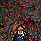
One thing we can notice is that black colouration of background not the face region. NST algorithm transfer is effective if the style reference image are highly texturized.