What is a Neural Network?
Think back to the first time you heard the phrase “neural networks” or “neural nets” — perhaps it’s right now — and try to remember what your first impression was. As an Applied Math and Economics major with a newfound interest in data science and machine learning, I remember thinking that whatever neural networks are, they must be extremely important, really cool, and very complicated. I also remember thinking that a true understanding of neural networks must be on the other side of a thick wall of prerequisite knowledge including neuroscience and graduate mathematics.
Through taking a machine learning course with Professor Samuel Watson at Brown, I have learned that three of the previous four statements are true in most cases — neural nets are extremely important, really cool, and they can be very complicated depending on the architecture of the model. But most importantly, I learned that understanding neural networks requires minimal prerequisite knowledge as long as the information is presented in a logical and digestable way. Indeed, this is part of the purpose of this article: to provide an easy-to-follow, yet insightful overview of what a neural network is. Another purpose of this article is to explain the advantages and disadvantages of the standard “vanilla” neural network versus recurrent neural networks (RNNs).
To accomplish these goals, I have split the article into three sections. The first section is an introduction to what neural networks are. The second section places neural networks (specifically vanilla neural networks) within a broader framework of machine learning models and comments on its advantages and disadvantages. The final section introduces a different type of neural network (RNN) and discusses how it mitigates some of the shortcomings of the standard vanilla neural network.
To the fellow DATA 1010 student, neural networks may just seem like one of many tools that we have at our disposal to model relationships between data. Despite spending extensive time studying vanilla neural networks, it can be easy to lose sight of how they fit into the broader context of neural networks and how neural networks fit into the broader context of machine learning. I believe it can be beneficial to take a step back, remind ourselves why the topic we are studying is important, and explore different types of neural networks to help us better fit our knowledge into a bigger picture. To the casual reader, I hope this article will be the wrecking ball of the “thick wall of prerequisite knowledge” and a valuable introduction to a few different types of neural networks. To any professional or anyone already familiar with this topic, I should apologize in advance for the simplistic nature of the article and lack of depth. Nonetheless, I hope this article can still be a useful summative resource and serve as an enjoyable read.
DATA 1010 Note: The first section of this article will primarily be a review of the vanilla neural networks that we have become familiar with in class. While I understand that the primary purpose of this article is to explore an adjacent topic, another goal of mine is to tell a good story that is useful to a larger audience. Therefore, I believe that it is important to provide some context and establish the broader framework within which we are working. That being said, feel free to start reading at the “Advantages and Disadvantages of Neural Networks” section where I begin to transition into my exploration of an adjacent topic (RNNs).
Setting the Scene
Let’s start with some context. Artificial intelligence (AI) is the branch of computer science concerned with programming machines to perform tasks that require human intelligence. Machine learning (ML) is a subset of AI that is focused on automating these processes, and the ability to learn and improve on past results without requiring user input. Neural networks (essentially synonymous to deep learning) are a subset of ML that are based on the structure of the brain.

It is also important to make the distinction between a biological neural network and an artificial neural network (ANN). A biological neural network is part of the actual neural system of the human body which consists of receptors, neural networks, and effectors. The primary component of the neural network is the neuron (pictured below) which consists of dendrites, somas, and axons. In this article, we will use “neural networks” to refer to ANNs and will not spend any time focusing on their biological counterparts. To be sure, ANNs are based on our understanding of biological neural systems so they really should not be thought of as separate entities. When we read a review on Amazon that starts with “This is the best…” we are likely to infer that the review is positive and will update our belief as we continue reading. We might be interested in simulating what our brain is doing in that process and can create a model that predicts the rating of a review, for example. In any case, neural networks allow us to emulate the complex capabilities of the brain so their importance should be obvious.

What are Neural Networks?
With that established, let’s get into the weeds of what a neural network is from a mathematical perspective. We illustrate the definition with a slightly modified example from class:
Suppose we have data for 1,000 houses in the Boston area represented on the x-y plane. The number of rooms of the house is the x-value, the distance from the nearest train station in miles is the y-value, and whether the house has a market value of over $250,000 (red points) or not (blue points) is color-coded. This is an example of a classification problem since we are interested in predicting which category a data point falls into given two features (x-value and y-value). If we were interested in predicting the exact market value then this would be a regression problem.
The essence of machine learning is that we can use a subset of the data (training data) to train our model. In this example we might use (say) 800 out of the 1000 data observations as training data. Suppose we are interested in constructing the most accurate linear model possible — a model that takes a data point (x,y) and calculates the quantity ax + by, predicting that the market value is over $250,000 if ax + by > c and less than $250,000 otherwise. We could imagine that a certain set of constants a1, b1, and c1 would result in 600 of the 800 houses being correctly classified and another set a2, b2, and c2 resulting in only 500 of the 800 houses being correctly classified. Our goal then is to find the values of a, b, and c that maximize the accuracy of the model on the training data. Then, we test the accuracy of our model on a separate subset of the original data, called the testing data. In this case, it would be logical to use the remaining 200 houses for testing purposes.
This type of problem could probably be solved with a variety of other machine learning techniques such as support vector machines since we would expect the data be somewhat evenly dispersed across the first quadrant of the x-y plane. However, if our data is oriented in a more complex way, such as in a spiral shape (pictured below), then many standard machine learning techniques may not have the complexity to sufficiently separate the data points (for example, a linear boundary would not get the job done).


Here is where neural networks are advantageous. We could imagine taking the data in the x-y plane and mapping them into the x-y-z plane as we see in the 3rd picture above. The data appear to orient themselves on the surface of a cube and we can see that they are easily separable now. We can use another function to map the points in 3D to the number line where points closer to 0 represent a higher likelihood of being red and points closer to 1 represent a higher likelihood of being blue. Then our model predicts “blue” if the value on the number line is greater than 0.5 and “red” otherwise. The model pictured above is able to separate our data perfectly.
To be more specific, we are interested in defining a composition of functions that takes a 2x1 vector (2D) as input, maps it to a 3x1 vector (3D), and then takes that 3x1 vector and maps it to a 1x1 vector (1D).

So how do we do this? In general, in order to transform a 2x1 vector to a 3x1 vector, we can multiply a 3x2 matrix by the 2x1 vector and add a 3x1 vector. For example, suppose our original point in the 2D graph is (3,2). We can represent that point as a 2x1 vector and multiply it by a 3x2 “weight matrix”. This process is illustrated below. In words the weight matrix is saying, the first component of the resulting 3x1 vector (before adding the bias vector) is comprised of 1 copy of 3 and -1 copy of 2, the second component is comprised of 2 copies of 3 and 0 copies of 2, and the final component is comprised of 2 copies of 3 and -4 copies of 2. The bias vector just shifts each component of the resulting 3x1 vector. Any function of this form (x -> Ax + b where A is the weight matrix and b is the bias vector) is called an affine function. Indeed, the one-dimensional analog of an affine function is just any function of the form f(x) = mx+ b.

Now to get our 3x1 vector to a 1x1 vector (going from 3D to 1D), we apply another affine function on the output from the last function. This time, our weight matrix is 3x1 and our bias vector is 1x1. To summarize, we transform a point in the x-y plane (3,2) to a point in the x-y-z plane (2,6,1) to a point on the number line (9) using a composition of affine functions (taking the output of the previous function as the input of the next.

The only problem with this approach is that a composition of affine functions is an affine function itself! For example, in the 1D case if we have a function f(x) = 2x + 7 and g(x) = 5x - 3, then f(g(x)) = 2(5x - 3) + 7 = 10x + 1. In other words, even though we could have several intermediate steps between our input and final output, we can always map the input to the final output directly using an affine function (in the above example, h(x) = 10x + 1 is equivalent to f(g(x)), so the composition of functions do not provide add any complexity in this case. Said differently, we could have gone directly from 2D to 1D in our previous example with a single affine function.
To fix this, we simply introduce an “activation function” at the end of each step. Activation functions are component-wise (meaning they are applied individually to every component of the vector) and allow us to introduce non-linearity into our composition of affine functions. One of the most common activation functions is sigmoid (shown below). Another common activation function is ReLU which maps negative numbers to 0 and positive numbers to themselves (f(x) = max(0,x)).

A neural network, then, is nothing but a composition of affine functions and component-wise activation functions. In our example, an example of a neural network might look something like this, where A1 and A2 are the two affine functions with the same weight matrices and bias vectors from above:

The only difference here is before we feed the vector (2,6,1) into the second affine function, we apply the sigmoid activation function on each component (2 becomes 1/1 + e^-2 which is 0.88 and so on). Again, the reason we do this is so that our composition of affine functions (A1 and A2) will not just result in an output that is linearly related to the input.
Here’s another example from class (pictured below). This time we start with a 3x1 vector input (1, -2, 3) and feed it into the first affine function with weight matrix W1 and bias vector b1 which sends it to 2D. Then we take the output (-3,4) and apply the ReLU activation function (negative numbers become 0, positive numbers stay the same) to get (0,4). Next we feed (0,4) into another affine function with weight matrix W2 and bias vector b2 and get an output of (3,1,2,-5). Applying ReLU again, we get (3,1,2,0) and that gets sent into a final affine function which yields (-1,-1). After applying the last affine function, we take our output just to be the output times the identity matrix. You can think of this as a special activation function which just keeps the output unchanged.

Note that this model has a different “architecture” (structure) than the first one. More specifically, the architecture is more complex since it involves a longer sequence of affine functions. We start with a 3x1 vector, map it to 2D, then to 4D, then back to 2D. We define a hidden layer to just be any layer or step that is not the input or output layer. So this neural network has more “hidden layers” than the last one.
Finally, we compare the output that our model spits out to the actual desired output that corresponds to our data. In our data, an input of (1,-2,3) produced an output of (3,2) and the model gave us an output of (-1,-1). We can use the squared norm of the difference between these outputs as a measure of how bad our model did (loss), and the goal is to minimize the loss of the model on the training data, on average. Let’s put it all together with a final example:

Above, we have 10 data observations, where each input (x,y) corresponds to an output z. Our goal is to construct a neural network that will allow us to predict z given (x,y). To do so, we split our data up into training data and testing data (5 each). Next, we use the training data to build a neural network that minimizes the average loss over the training data. That is, we want our model to do the best it can at returning outputs of 5, 9, 4, 3, and 5, respectively when we feed it the 5 training data inputs. In other words, we want to find the optimal weight matrices and bias vectors (that make up each affine function) that will cause the outputs of the model to be as close as possible to the actual outputs.
Once we have determined the best weight matrices and bias vectors, we have a neural network that is ready to be tested on the testing data. We feed the 5 inputs of the testing data into the model we just constructed and see how close the model’s outputs are to the actual desired outputs. If we did a good job, then our average loss should be small.
To be clear, just because we can construct a model that performs well on training data does not mean the model is good in general. Keep in mind that the way we construct neural networks is to maximize their performance on the training data. We test the model on a separate set of data since the training data may not be a good representation of the overall population.
In real world scenarios, we might be given a sample of 100,000 data observations of which we randomly select 80,000 observations to train our model on. After training, our model will be the one that performs the best on the 80,000 observations that we trained it on (in other words, the weight matrices and bias vectors of our model will produce the lowest possible average loss when we consider training data only). Since we have such a large sample and the training data was randomly selected, we are confident that the 80,000 training observations are representative of the general population (which could be much greater than 100,000). Since we do not have access to any other data outside the sample of 100,000, the best we can do for now is just test the model on the remaining 20,000 observations. That being said, the overall goal is to use the model on future data.
The table below serves to summarize our discussion about what a neural network is and how to construct one:

Wait, so how exactly do we determine the best values for the weight matrices and bias vectors? If your initial thought is trial and error, you are not far off. The general idea is we start with certain values in these weight matrices and bias vectors and slightly change one value at a time and see if that makes our output more or less accurate on average. This is the essence of a partial derivative, which answers the question “how does my output respond to a tiny change in my input, holding all other inputs constant?” If we had a way to calculate the partial derivatives of all the values of the weight matrices and bias vectors, then we can use gradient descent to move our values in the direction of greatest accuracy improvement in tiny steps until our average loss is below some threshold. We will not spend time discussing the details of training neural networks in this article but hopefully this paragraph provides some basic intuition.
Advantages and Disadvantages of Neural Networks
The neural networks that we just discussed are known as standard or vanilla neural networks. Here, we also introduce the term “feed-forward network” which just refers to a network where the nodes do not ever form a cycle; the inputs feed into some nodes which feed into new nodes and so on until we reach the output. Think of “feed-forward” as traveling from left to right. A vanilla neural network is just a feed-forward network, usually one with at least one hidden layer like the ones we covered in the previous section and the example pictured below.

The last concept we need to introduce before diving into advantages and disadvantages is underfitting versus overfitting. Recall that when we train a model we want to minimize the average loss over the training data which is typically a subset of data observations we have at our disposal. The data observations we have at our disposal are a subset of the entire population from which the data was sampled, and the goal of any model is to represent the overall population accurately. Below, we have 3 different models corresponding to the same training data. The training data seem to follow some sort of upward quadratic U-shape, and the middle model does a good job of fitting the general shape of our data. Even though the sample size is not particularly large, we feel pretty confident that the general population follows some sort of quadratic shape.
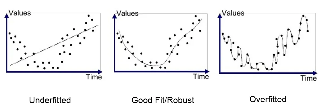
Overfitting refers to when we do “too good of a job” and introduce complexity that is unlikely to accurately represent the population. Our model on the right does a really good job at minimizing the average loss over the training data since the model basically passes through every point. However, introducing such a higher degree of complexity does not do us any good when it comes to making conclusions about the entire population, since the entire population is unlikely to follow such a radical shape.
We need to be careful when we say that the goal of training is to minimize the average loss over the training data. If our model takes those instructions too literally, we end up overfitting the data. A logical way to prevent overfitting is to introduce some constraints about the form our model can take. The most common example is linear regression which basically says “do the best you can at minimizing average loss but you are only allowed to use a straight line”. Linear regression can help us avoid overfitting but sometimes can be a little too restrictive and cause us to actually underfit the data. As you can see above, the model on the left seems a little better than the one on the right but is missing out on some of the desired complexity that the middle model offers.
Therefore, we need to select our model based on many factors including the complexity of the data. Linear regression works brilliantly in many scenarios but when the data is more quadratic (such as the example above) or in a spiral shape (such as a prior example), the restrictive assumptions of linear regression limit our capability to model the data accurately.
Five different ML techniques are pictured below, each of which have their pros and cons depending on the way the data is distributed.

The main advantage of neural networks is their almost limitless flexibility of learning patterns that no other ML model can learn. If our data is relatively simple, we can use a neural network with a simple architecture (perhaps mapping directly (say) from 2D to 1D). If our data is more complicated, we can increase the complexity of our architecture. The ability to calibrate the structure of our model to our needs makes neural networks the most robust ML model. There are very few problems that neural networks cannot solve.
The main disadvantage of neural networks is that they are expensive in many different senses of the word. To start, most neural networks require tons of data to produce desirable results and are computationally expensive compared to their counterparts. Also, even though the freedom of choosing a structure is a good thing, picking a good architecture (the amount of hidden layers, how many dimensions we need, etc.) can be challenging. Therefore, the development process of neural networks tends to be fairly long and complicated. Another disadvantage is the “black box” nature of most neural networks, especially ones with multiple hidden layers. Even though neural networks tend to be extremely accurate, we often cannot make sense of how the model arrived at its conclusion or assign interpretations to numbers since most of the magic is happening within a huge maze of affine functions.

To illustrate some of these advantages and disadvantages with an example, consider the digit recognition model below. Our input is a 28x28 pixel image and our output is a digit from 0–9. Each of the 784 (28²) pixels represents an input with a value from 0 (black) to 1 (white) indicating the intensity of that pixel (for example, most of the 784 pixels of the digit 7 pictured below will have a value of 0 corresponding to black, some will have a value close to 1 corresponding to the brightest part of the seven, and the pixels at the edge will have values between 0 and 1). In other words, our input is a 784x1 vector and our output is a 10x1 vector. We have two hidden layers (each with 16 nodes) and apply some unknown activation function.

So how many parameters are at play here? We know that the first affine function will transform our 784x1 input vector to a 16x1 vector which requires a 16x784 weight matrix and a 16x1 bias vector. After applying some activation function, the second affine function will transform a 16x1 vector to another 16x1 vector, requiring a 16x16 weight matrix and a 16x1 bias vector. After applying some activation function again, the final affine function will transform a 16x1 vector to a 10x1 vector, requiring a 10x16 weight matrix and a 10x1 bias vector. The model will then choose the component of the final 10x1 output vector that has the largest value as its prediction. So in the above example, the 8th component of the 10x1 vector had the largest value so the model predicts “7”.
In total, we have three weight matrices (16 x 784, 16x16, 10x16) and three bias vectors (16x1, 16x1, 10x1) which correspond to 13,002 different values that we have to determine via the training process! It makes sense now that neural networks require a huge amount of training data in order to determine the optimal value for each of its parameters, and this digit recognition network is on the simpler side. That being said, the task of recognizing digits (a 10 category classification problem) exceeds the capabilities of most other machine learning techniques. The tradeoff between the power of a neural network and its high cost is on full display in this example.
While neural networks clearly have their drawbacks, most people would agree that the benefits that they offer far exceed their negatives. For one, even though neural nets tend to be expensive, they often are the only viable option we have when analyzing highly complicated data. In addition, we have complete control over the type of neural network we choose to use as well as its architecture, so neural networks can solve problems of any complexity. The following section discusses why even the vanilla neural network might be too simple in some cases and how recurrent neural networks mitigate that shortcoming.
Recurrent Neural Networks
The key idea behind vanilla neural networks is that all of the inputs are independent. This bodes well for tasks such as pattern recognition (which includes digit recognition, image recognition, data classification, etc.) where all of our data are fed into the neural network simultaneously. For example, in the digit recognition example we simultaneously input the 784 pixel values of an image and the vanilla neural net was trained to detect distinguishing features of each of the 10 digits.

A clear shortcoming of vanilla neural networks is their inability to make predictions about sequential data. Because all of the data is inputted at the same time, there is no notion of time or dependence. Tasks such as predicting the price of a stock given the previous 90 days’ closing prices and speech recognition which relies on which word is most likely to follow previous words (Siri) are outside of the capabilities of these basic neural networks.
Recurrent neural networks mitigate this shortcoming by taking inputs one at a time. Instead of inputting all of the data (x0, x1, …, xt) at the beginning, the RNN below starts by inputting just x0, feeding it through a hidden layer A and returning h0 as output. The key difference is when the next data point x1 is inputted, it’s hidden state is combined with the hidden state of x0 to produce h1. Therefore, h1 depends on x0 and x1, h2 depends implicitly on x0, x1, and x2, and so on where each output depends on all previous inputs.

Let’s rigorize this with an example. Suppose our goal is to create a character level language model that autocompletes a word. In order to do so, we need to figure out a good way to represent letters as numbers.
A logical way to vectorize the letters of the alphabet is to let each letter be represented by a 26x1 vector with a 1 in the component corresponding to that letter and 0’s in the remaining 25 components.

We will follow a simplified version of that method by assuming that our pool of letters only consists of the letters H, A, P, and Y. We would like our model to perform as follows:

In words, we want to input the 4 letters H, A, P, P in that order and would like the model to return A, P, P, Y in that order. More specifically, we want our model to predict the letter A when given the letter H, predict the letter P when given HA, predict P when given HAP, and predict Y when given HAPP. The horizontal arrows in the middle demonstrate that the outputs (besides the first one) depend on all previous inputs.
Note that in all diagrams below there is a typo. “4x3 W3a” and “4x3 W4a” should say “4x3 W3b” and “4x3 W4b”

Each of the vertical arrows still represent affine functions. This time we do not consider bias vectors (in other words, assume the bias vectors are all 0) but the process can easily be generalized to include bias vectors. We know our input vector is a 4x1 vector and it probably makes sense for our output vector to also be 4x1 so we can translate it back to one of the 4 letters {H, A, P, Y}. We choose to transform the 4x1 vector to a 3x1 vector in the hidden layer and then back to a 4x1 vector for the output layer. This involves multiplying our input by a 3x4 weight matrix and then the result of that by a 4x3 weight matrix. In total, we will have four 3x4 weight matrices and four 4x3 weight matrices.
Of course, we still need to choose an activation function between the two affine functions, otherwise we will not be able to introduce non-linearity. Being able to introduce non-linearity is important because like we discussed above, having your output be linearly related to your input limits the complexity of our model.

We now demonstrate the process of inputting the first vector using code:

We first define the activation function to be sigmoid, initialize the input vector H, and make a random 3x4 weight matrix W1a.
Next, we apply the affine function corresponding to the weight matrix W1a to our input vector H (remember, no bias this time).
Then, we apply the activation function to each component of the resulting output.
Next, we create a random 4x3 weight matrix that corresponds to the second affine function and apply the second affine function on the previous output.
As desired, our output is a 4x1 vector and we can take the largest component to be 1 and the remaining 3 components to be 0 in order to translate it back to a letter. In this case, we actually get the letter A as output by pure chance.
We update our diagram accordingly:

Because that was the first input, there was no dependence on previous letters and the process we followed was identical to that of a vanilla neural network. We will see now that the second output depends (implicity) on both the first and second inputs.
Notice how we still haven’t defined what the horizontal arrows mean. Normally they would represent yet another affine function but for the purposes of this demonstration let’s just assume they represent addition. In other words, once the letter A (0,1,0,0) gets multiplied by the 3x4 weight matrix (W2a), we would like to add the resulting 3x1 vector to (0.86, 0.62, 0.29). Let’s do this with code again:

We initialize the second input A, and define random weight matrices W2a and W2b that correspond to the affine functions pictured in the diagram.
Next, we apply the first affine function (W2a) on the input vector A and add the resulting 3x1 vector with the 3x1 vector from the previous hidden layer.
Then, we apply the activation function component-wise on the new 3x1 vector and apply the second affine function that corresponds to W2b on the result.
We end up with a 4x1 vector whose first component is largest so that corresponds to an output of (1,0,0,0) or H. We update our diagram accordingly:

The crucial takeaway is that the vector (0.94, 1.54, 0.63) is the sum of (0.86, 0.62, 0.29) and the 3x1 vector that results from multiplying W2a and (0,1,0,0). In other words, the hidden layer of the second input depends on both H and A so we have introduced sequential dependence.
We follow the same process for the two P’s and the completed diagram is shown below:

We can see that our resulting model does a poor job of predicting the next letter, only getting one out of four correct. That shouldn’t come as a surprise though, given our eight weight matrices were randomly generated. Training the neural network, like in the vanilla case, involves finding the optimal values for each of the eight weight matrices. In our case, we would like our model to return as many correct letters as possible, and there is good reason to believe that we can do better than one out of four.
Generalizing this example, we could do something similar with all 26 letters and data corresponding to hundreds of thousands of words. After training our model on a subset of those words, a successful model would be able to determine the most likely letter to follow a sequence of letters. Remember, the dependence of previous letters comes from the hidden layers. In our simple example, we just added the vectors but more complex functions are usually involved in that step.
What are the shortcomings of RNN? They tend to forget the previous inputs pretty quickly like the below animation shows. The circles represent the hidden layers and we can see that by the time you are at the fifth input, the hidden layer barely depends on the first input. We can resolve this issue using long short term memory (LSTM) networks but that is a story for another article.

Conclusion
The take home message here is there is no silver bullet in machine learning. We discussed the concept of overfitting versus underfitting and demonstrated how every model is prone to either lacking complexity to solve certain problems or being too computationally expensive or inefficient. The value of having a rigorous understanding of various machine learning techniques cannot be overstated; it will equip you with a robust skillset to tackle various interesting and tangible problems. If you have prior experience in this field, I encourage you to continue to deepen your understanding of neural networks and other machine learning techniques. If this is your first exposure to ML or even AI in general, hopefully I have convinced you that neural networks is a good place to start and piqued your interest to explore more. I have included a picture of the most common types of neural networks below:

If I had the time to explore each of these neural networks one by one and write an article for each of them I would, but articles like this one exist all over the place including right here on Medium. In fact, much of my understanding of RNNs was developed from browsing other Medium articles which demonstrates how powerful an engaged academic community can be.
That wraps up our discussion about neural networks. I hope that you will leave this article with a newfound interest and understanding of how these incredible mechanisms work. Moreover, I hope that you will leave this article with more questions than you had coming in. This article is not meant to be a comprehensive guide to neural networks. Rather, it is intended to place neural networks into a digestible and coherent framework and serve as a springboard to future discoveries.
Thank you for reading and please feel free to email me if you have any questions (ethan_huang1@brown.edu).
