CNNs from a Biological Standpoint — Biological Computer Vision (1/3)

This post is the first of my three-part series on comparing computer vision architectures to the human visual system — Biological Computer Vision.

Convolutional Neural Networks (CNNs) are the industry standard when it comes to AI tasks related to images — Computer Vision. CNNs were a considerable upgrade from typical Artificial Neural Networks (ANNs) for Computer Vision tasks dating back all the way to 1998. CNNs were specifically designed for tasks dealing with visual information with heavy initial inspiration from animal visual pathways. Today, CNNs have a lot of application in fields like Natural Language Processing and Drug Discovery but still stay true to its roots in computer vision.

A brief history of CNNs

ANNs — a Black Box Summary

This article assumes the knowledge of Artificial Neural Networks (ANNs). If not, here is a quick black-box explanation. An ANN is modelled after the human brain and is made up of layers of computational units called neurons. These neurons are connected to neurons in other layers with connections that have specific weights. Data is passed to the input layer, through the hidden layers and finally to the output layer that gives us our prediction. Due to fancy mathematical properties of neurons and weights, the Neural Network is a Universal Approximator which means that the network can represent any mathematical function which essentially implies that it can solve any problem thrown at it with the right connection weights. These connection weights are ‘learned’ (hence the name Machine Learning) in the training phase of the modelling process. The more hidden layers there are in an ANN, the ‘deeper’ it is said to be (hence the name Deep Learning) and the easier it is (usually) to approximate the required function. Here is a useful resource to learn the intricacies and magic of ANNs.

A simple ANN with one hidden layer. The connections between the neurons have weights specific to them (not pictured here) that help the function approximation process. via github

Problems with the predecessor

Artificial Neural Networks were the de-facto standard for almost every Artificial Intelligence task back in the day. For computer vision, engineers and researchers relied on small images being fed into the network. This is because the weights of every connection in the network had to be calculated using an algorithm called backpropagation. Let’s say we have a 10x10 grayscale image as an input for our network, this would be translated into a 100 dimension vector for the input layer. Let’s assume the first hidden layer of the network has 2 neurons, this would mean that we need to estimate the weights of 200 weights (100 weights per neuron since there are 100 input neurons) which seems quite computationally expensive. Now imagine a more realistic scenario where we have a much larger image, say 500x500 that we translate into a 250,000 dimension vector for the input layer. Now, we will have to estimate 250,000 weights per neuron in the first hidden layer. You can see how this is ridiculously computationally expensive especially considering the fact that ANNs have multiple hidden layers. For this reason, researchers started looking for more efficient networks to perform computer vision tasks.

Each of these connections have weights that are crucial for inference which is estimated repeatedly using backpropagation. In a fully connected network, each neuron in the previous layer is connected to each neuron in the next layer. TLDR: Lot of weights and consequently, lot of calculations! Via researchgate

Another aspect of vision that ANNs struggled with is the loss of contextual information. Images tend to be heavily contextually correlated. For example in an image of a beach, a blue pixel will be close to other blue pixels (the ocean or the sky) whereas a brown pixel will be closer to other brown pixels (the sand). The ANNs were not leveraging this useful contextual information that we, as humans seemed to be using.

Leveraging the fact that there are a lot of patches in the image where blue pixels are close together and brown pixels are closer together should make it easier for a network to classify that this is an image of a beach. How could an ML algorithm do this? Via livescience

Inspiration to improve ANNs

Researchers turned to literature on animal visual pathways to find an ML architecture that was more efficient for image processing and leveraged contextual information. Very popular research by Hubel and Wiesel showed that two types of neurons (heavily generalised here) are mainly responsible for visual perception in animals — Simple Cells (S Cells) and Complex Cells (C Cells). S Cells activate when they identify basic shapes in a small, fixed area regardless of orientation whereas C cells have larger receptive fields and can identify shapes even if they are not in their typical positions in the field.

These Simple and Complex Cells and their ability to identify shapes of various orientations from larger receptive fields are what inspired ML researchers to develop Convolutional Neural Networks.

How do CNNs work?

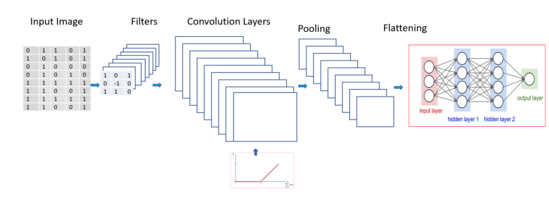
The architecture of a typical CNN for image classification involves the Feature Extraction part and the Classification part. The feature extraction part is what makes the CNN stand out from your old-school ANNs. This component hinges on the use of filters to detect features from patches of the image. These filters are analogous to the C cells from the previous section!

Filters, Features and Feature Maps

Features are what make an image well, a meaningful image. Common features when you are classifying images are edges, vertical or horizontal lines, basic shapes, etc. These features make up an image. Some images have more of some features than others. For example, images of a zebra will have more features of vertical lines than say images of a panda. Since features cannot be found at the pixel-level, patches or sections of an image consisting of multiple pixels are ‘scanned’ for features. This is the kind of information we leverage when using CNNs to classify images.

Taking regions of the image into account using overlapping patches directly addresses the problem of not leveraging contextual information in previous ANNs.

CNNs’ classification process starts with the image being ‘scanned’ for specific features using filters. These filters then build a feature map — a representation of the occurrence of these features in that image. These feature maps undergo further operations called pooling that conserves only the important information in the feature maps and reduces their sizes to reduces the number of computations in the network. These pooled feature maps are fed into the input layers of the classification part to come up with scores for each class (if a CNN is classifying images into vehicles, the classes would be each vehicle) in the problem as the output.

The CNN’s architecture has hidden layers which extract features in the image with the help of kernels to build feature maps. The feature maps are then fed as flattened vectors into a classification network. The classification network returns with the likelihood of the vector being each class. The class with the highest likelihood will be the prediction by the network. via Miro

Where does the Convolution in Convolutional Neural Networks come in?

In order to build a feature map, we slide the filter across the image multiple times to search for the features. The filter is nothing but a matrix of weights that correspond to the feature it is filtering for. At each patch, the CNN finds the dot product of the pixels in the patch and the respective weights of the filter as pictured below. The result is then used to build the feature map. The rest of the values in the feature map will be populated as the filter iterates through the other patches of the image. This process of applying the filter to an input image patch-by-patch to obtain the feature map is called convolving the input image with the filter (hence the name of CNNs!).

In this example, we are looking for a diagonal edge feature in an image. The filter is convolved with each patch of the input image to build a feature map. via StatQuest

Feature Maps and Visual Cells

So we know that the feature map tells us where and ‘to what extent’ the corresponding features occur in the input image. This information is very similar to what Hubel and Wiesel’s cells tells our visual system. S cells are excited when a specific shape is shown to it at a specific location at any orientation. C cells are excited when a specific shape is shown to it at any location in its excitatory field. Therefore the S-cells are orientationally invariant and the C-cells are spatially invariant. These two invariance properties are conserved by the CNN as the filters are able to mathematically observe the presence of a feature despite its orientation and the spatial location thanks to the dot product computation and the sliding of the filter through the image respectively. The stimuli that excite certain S and C cells are analogous to the features in the CNNs. The excitations of the S Cells and C Cells finally undergo summations and integrations to form a visual representation in the animal visual pathways — very similar to a feature map.

It is still unclear what constitutes a complex cell but it is theorised that a complex cell could draw inputs from itself, other C cells and simple cells as well. via researchgate

Further Technicalities and Operations

The feature maps undergo further operations before being input into the classification network. An activation function (typically ReLU) is first applied to the feature maps to introduce non-linearity into the system which is a common aspect of Artificial Neural Networks. The output of the activation the undergoes a process called pooling (typically Max pooling) which essentially downsamples the feature map to a smaller size while conserving information about the spatial allocation of features. These operations are pictured in the figure below.

Pooling (along with the use of patches instead of filters) directly solves the problem of a large number of computations for images in previous ANNs

Visual representations of the effect filters, activation functions and pooling have on an image patch in CNNs. via statquest

The pooled feature maps are fed into the input layers which then handle the classification problem like how any typical ANN handles it but now, both problems of efficiency and contextual information have been solved.

It is important to note that the filters are learned during the training phase of the network. The weights in each filter are randomly assigned at the beginning and during training, the weights are estimated using backpropagation, just like how weights of connections are learned in ANNs. Once the training phase is complete, the weights of each filter should correspond to the features present in the images the network was trained with.

Convolutional Neural Networks have their roots firmly planted in the origins of understanding visual perception in animal visual pathways. The inspiration was then combined with the engineering of pre-existing Artificial Neural Networks to produce the state-of-the-art architectures of CNNs that are able to exceed human performance on visual processing tasks.

This is part 1 of my 3-part series on how Computer Vision architectures take inspiration from animal visual systems. I will be tackling the newer, Visual Transformers in the next article and then compare the two leading architectures to find out which is more like human visual processing.