Hash Tables, Hashing and Collision Handling
In continuation to my data structure series, this article will cover hash tables in data structure, the fundamental operations of hash tables, their complexities, applications of hashing, the various types of collisions and how to handle them. You can read the other topics in this series:
Before going into Hash tables, we need to understand the concept of hashing and hash functions.
So what is Hashing?
It is the process of converting a given key into another value, with the help of a hash function. A hash function is nothing but a mathematical algorithm which helps generate a new value for a given input. The result of a hash function is called a hash, or a hash value.
Let’s quickly learn what properties a hash function should have, to be called a good hash function:
- Efficiently computable
- Should uniformly distribute the keys
We can always write our own hash functions but it is recommended not to, for there are really good hash functions already out there.

Hash Tables
A hash table is a data structure that implements an associative array abstract data type, a structure that can map keys to values. A hash table uses a hash function to compute an index, also called a hash code, into an array of buckets or slots, from which the desired value can be found. — Wikipedia
In a hash table, every key is unique. We should use this data structure when the ordering and sorting of data is not needed, because the order of data is not retained here.
Hash tables must support 3 fundamental operations:
- Insert(key,value) -> Adds an item to the hash table.
- get(key) -> Fetches the value with the help of the given key.
- delete(key) -> Removes a value with the help of the given key.
These operations should ideally execute in O(1) time. By calculating the index of a given key very fast, hashing on average ensures a constant time decision on where to insert into or delete/fetch from, in the hash table. However, in the worst case, these operations can be of O(n) but we will discuss that a bit later.
How does hashing help achieve such fast storing, removing and searching of data?
A hash table stores data in key-value form. During insertion for a provided key, a hash function converts the key into an index of the hash table. The value is then stored at that index. The hash function can produce an index that has already been used in the table, which is called a collision. We will discuss how to handle collisions soon. It is due to this hash function that we are directly computing the location of a data in the table that ensures the fast operational times of this data structure.
Applications of Hashing
- Implementing hash table, hash map, python’s dictionary, unordered set
- cryptography: A cryptographic hash function produces output from which reaching the input is almost impossible. This property of hash function is called irreversibility. Example of a cryptographic hash function is the popular SHA256 algorithm.
- Password verification
- Compiler operations
- Pattern searching algorithms like Robin Carp algorithm
Collisions and How to Handle Them
Two or more keys can generate same hash values sometimes. This is called a collision. A collision can be handled using various techniques.
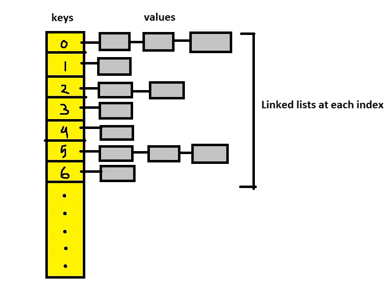
Separate Chaining Technique
The idea is to make each cell of the hash table point to a linked list of records that have the same hash function values. It is simple but requires additional memory outside the table. In this technique, the worst case occurs when all the values are in the same index or linked list, making the search complexity linear (n=length of the linked list). This method should be used when we do not know how many keys will be there or how frequently the insert/delete operations will take place.
To maintain the O(1) time of insertions, we make the new value as head of the linked list of the particular index.
I am providing the code of a generic hash table implementation with separate chaining technique, using an ArrayList of linked lists.
// this is the custom generic node class
public class HashNode<K,V> {

    K key;
    V value;
    HashNode<K,V> next;

    public HashNode(K key,V value){
        this.key = key;
        this.value = value;
    }
}
public class CustomHashMap<K,V> {
private ArrayList<HashNode<K,V>> bucketArray;
private int numBucket; //current capacity of list
private int size; // current size of list
public CustomHashMap(){
bucketArray = new ArrayList<>();
size = 0;
numBucket = 10;
//we create empty chains
for(int i=0;i<numBucket;i++){
bucketArray.add(null);
}
}
public int getSize(){
return size;
}
public boolean isEmpty(){
return size==0;
}
private int getBucketIndex(K key){
int hashCode = key.hashCode(); //built in java hash func
int index = hashCode%numBucket;//mod to traverse circularly
return Math.abs(index); // since the key could be negative
}
public V remove(K key){
//we find the required index
int bucketIndex = getBucketIndex(key);
HashNode<K,V> head = bucketArray.get(bucketIndex);
HashNode<K,V> prev = null;
while(head!=null){
if(head.key.equals(key)){
break;
}
prev = head;
head = head.next;
}
if(head==null){
return null;
}
size--;
if(prev!=null){
prev.next = head.next;
}
//here we are handling if key is first element when prev WILL be null
else{
bucketArray.set(bucketIndex,head.next);
}
return head.value;
}
public V get(K key){
int bucketIndex = getBucketIndex(key);
HashNode<K,V> head = bucketArray.get(bucketIndex);
while(head!=null){
if(head.key.equals(key)){
break;
}
head = head.next;
}
if(head==null){
return null;
}
return head.value;
}
//add key value pair to hash table
public void add(K key, V value){
int bucketIndex = getBucketIndex(key);
HashNode<K,V> head = bucketArray.get(bucketIndex);
//if key already exists, we update the value
while(head!=null){
if(head.key.equals(key)){
head.value = value;
return;
}
head = head.next;
}
//insertion at head for o(1)
size++;
HashNode<K,V> newNode = new HashNode<>(key,value);
head = bucketArray.get(bucketIndex);
newNode.next = head;
bucketArray.set(bucketIndex, newNode);
//now to check for the load factor
if((1.0*size)/numBucket>=.7){
size = 0;
ArrayList<HashNode<K,V>> temp = bucketArray;
bucketArray = new ArrayList<>();
numBucket = 2*numBucket;
//we create the chains again first
for(int i=0;i<numBucket;i++){
bucketArray.add(null);
}
//finally we copy from old to new
for(HashNode<K,V> node:temp){
while(node!=null){
//recursively
add(node.key,node.value);
node = node.next;
}
}
}
}
}Load Factor = number of items in the table/slots of the hash table. It is the measure of how full the hash table is allowed to get before it is increased in capacity. For dynamic array implementation of hash table, we need to resize when load factor threshold is reached and that is ≤0.7 ideally.
Open Addressing technique
In this method, the values are all stored in the hash table itself. If collision occurs, we look for availability in the next spot generated by an algorithm. The table size at all times should be greater than the number of keys. It is used when there is space restrictions, like in embedded processors.
Point to note in delete operations, the deleted slot needs to be marked in some way so that during searching, we don’t stop probing at empty slots.
Types of Open Addressing:
- Linear Probing: We linearly probe/look for next slot. If slot [hash(x)%size] is full, we try [hash(x)%size+1]. If that is full too, we try [hash(x)%size+2]…until an available space is found. Linear Probing has the best cache performance but downside includes primary and secondary clustering.
- Quadratic Probing: We look for i²th iteration. If slot [hash(x)%size] is full, we try [(hash(x)+1*1)%size]. If that is also full, we try [(hash(x)+2*2)%size]…until an available space is found. Secondary clustering might arise here and there is no guarantee of finding a slot in this approach.
- Double Hashing: We use a second hash function hash2(x) and look for i*hash2(x) slot. If slot [hash(x)%size] is full, we try [(hash(x)+1*hash2(x))%size]. If that is full too, we try [(hash(x)+2*hash2(x))%size]…until an available space is found. No primary or secondary clustering but lot more computation here.
Don’t worry if the mathematical notation confuses you. Let us walk through an example case. For a hash table of size 10, say our hash function hash(x) calculates index 3 for storing the data. So here, [hash(x)%10]=3. If index 3 is already full, linear probing gives us [3%10+1]=4 and we store the data at 4th index if not filled already. Similarly, quadratic probing gives us [(3+1*1)%size]=4. Let’s go a step further here, and assume the 4th index is now filled too. Quadratic probing then will calculate [(3+2*2)%10]=7th index to be used for storing the data. Try and find out what index double hashing would calculate.
I am providing the code of a hash table implementation with linear probing technique, using two arrays. This implementation can be tweaked to use quadratic probing or double hashing as well, I will leave that to your curiosity.
public class LinearProbing{
    private String [] keys;
    private String [] values;
    private int size;
    private int capacity;

    public LinearProbing(int capacity){
        keys = new String[capacity];
        values = new String[capacity];
        this.size = 0;
        this.capacity = capacity;
    }

    public void makeEmpty(){
        size = 0;
        keys = new String[capacity];
        values = new String[capacity];
    }

    public int getSize(){
        return size;
    }

    public int getCapacity(){
        return capacity;
    }

    public boolean isFull(){
        return size==capacity;
    }

    public boolean isEmpty(){
        return size==0;
    }

    private int getHash(String key){
        return Math.abs(key.hashCode()%capacity);
    }

    public void insert(String key,String value){
        if(isFull()){
            System.out.println("No room to insert");
            return;
        }
        int temp = getHash(key);
        int i = temp;
        do{
            if(keys[i]==null || keys[i].equals("DELETED")){
                keys[i] = key;
                values[i] = value;
                size++;
                return;
            }
            if(keys[i].equals(key)){
                values[i] = value;
                return;
            }
            i = (i+1)%capacity;
        }while(i!=temp);
    }

    public String get(String key){
        int i = getHash(key);
        while(keys[i]!=null){
            if(keys[i].equals(key)){
                return values[i];
            }
            i = (i+1)%capacity;
        }
        return "not found";
    }

    public boolean contains(String key){
        return get(key)!=null;
    }

    public void remove(String key){
        if(!contains(key)){
            return;
        }
        int i = getHash(key);
        while(!keys[i].equals(key)){
            i = (i+1)%capacity;
        }
        keys[i] = values[i] = "DELETED";
        size--;
    }
}
If it was a dynamic array implementation, we would have to check the load factor at some point of removal or insertion and take necessary steps. However, for simplicity of understanding I have used plain arrays here. Don’t worry about the “DELETED” flags, because if you look closely, they are overridden during insertions. Note that, there are other ways to implement the hash table with linear probing, feel free to explore them! It will only sharpen your understanding.
Additional Hashing Knowledge
Perfect Hashing: A hash function that maps each different key to a distinct integer value or index of a table. Usually, all possible keys must be known beforehand. A hash table that uses perfect hashing has no collisions. It is also known as optimal hashing.
Distributed Hashing: Used to store big data on many computers. Consistent hashing is used to determine which computers store which data. Read more about consistent hashing here.
Conclusion
In this article, I have tried to get the reader up and running with the fundamental aspects of hashing and hash table data structure. Like I repeat in every article, to master any data structure we need to solve problems with it. Head over to LeetCode, HackerRank and GeekForGeeks to find many problems on the topic and start solving them to earn that mastery. Also, please note that the code provided above can always be optimized and has been written based on certain assumptions. I hope you have learned something from this write up. Thanks for reading!