
Robotic Arm Gripper trained to hold object using Deep Reinforcement Learning
Implementation of Deep Deterministic Policy Gradient (DDPG) Algorithm to train a Robotic Arm to consistently reach out to dynamically moving target location in Single-Agent Reacher Unity ML-Agent Environment

A brief introduction to the Problem Statement
Using a Single-Agent version of the Multi-Agent Reacher Unity ML-Agent environment, the objective of the project is to train a double jointed Robotic Arm Agent which can reach out to target locations (green sphere revolving around the robotic arm) to maintain its position at the target location for as many timesteps as possible even as the target moves dynamically changing its position real-time. A reward of + 0.1 is provided for each timestep that the robotic arm agent is at the goal location. The agent’s observation space consists of 33 variables corresponding to position , rotation , velocity and angular velocities of the double-jointed Robotic Arm. The agent’s action space is continuous. Each action ia a vector with 4 numbers (size:4) corresponding to torque applicable to two joints of the Robotic Arm. Every entry in action vector should be in the range of (-1,1). The task is episodic, and in order to solve the environment, the agent must get an average score of +30 over 100 consecutive episodes.
Results Showcase :
An Untrained Robotic Arm Agent taking random actions failing to reach out to the moving Target location

A Trained Robotic Arm Agent consistently reaching out to the moving Target location
State Space :
The observation space consists of 33 variables corresponding to position , rotation , velocity and angular velocities of the double-jointed Robotic Arm
Action Space :
The Action Space is continuous. Each action is a vector with 4 numbers (size:4) corresponding to torque applicable to two joints of the Robotic Arm. Every entry in action vector should be in the range of (-1,1)
Solution Criteria :
Only one robotic arm agent is present and the task is episodic.
The environment is considered as solved when the agent gets an average score of +30 over 100 consecutive episodes.
NOTE:
The current implementation has been done only for the Single-Agent Reacher Environment.
Relevant Concepts
This section provides a theoretical background describing current work in this area as well as concepts and techniques used in this work.
a) Reinforcement Learning: Reinforcement Learning has become very popular with recent breakthroughs such as AlphaGo and the mastery of Atari 2600 games. Reinforcement Learning (RL) is a framework for learning a policy that maximizes an agent’s long-term reward by interacting with the environment. A policy maps situations (states) to actions. The agent receives an immediate short-term reward after each state transition. The long-term reward of a state is specified by a value-function. The value of state roughly corresponds to the total reward an agent can accumulate starting from that state. The action-value function corresponding to the long-term reward after taking action a in state s is commonly referred to as Q-value and forms the basis for the most widely used RL technique called Q-Learning
b) Temporal Difference Learning : Temporal Difference learning is a central idea to modern day RL and works by updating estimates for the action-value function based on other estimates. This ensures the agent does not have to wait until the actual cumulative reward after completing an episode to update its estimates, but is able to learn from each action.
c) Q-Learning : Q-learning is an off-policy Temporal Difference (TD) Control algorithm. Off-policy methods evaluate or improve a policy that differs from the policy used to make decisions. These decisions can thus be made by a human expert or random policy, generating (state, action, reward, new state) entries to learn an optimal policy from.
Q-learning learns a function Q that approximates the optimal action-value function. It does this by randomly initializing Q and then generating actions using a policy derived from Q, such as e-greedy. An e-greedy policy chooses the action with the highest Q value or a random action with a (low) probability of , promoting exploration
as e (epsilon) increases. With this newly generated (state (St), action (At), reward (Rt+1), new state (St+1)) pair , Q is updated using rule 1.This update rule essentially states that the current estimate must be updated using the received immediate reward plus a discounted estimation of the maximum action-value for the new state. It is important to note here that the update is done immediately after performing the action using an estimate instead of waiting for the true cumulative reward, demonstrating TD in action. The learning rate α decides how much to alter the current estimate and the
discount rate γ decides how important future rewards (estimated action-value) are compared to the immediate reward.
d) Experience Replay: Experience Replay is a mechanism to store previous experience (St, At, Rt+1, St+1) in a fixed size buffer. Minibatches are then randomly sampled, added to the current time step’s experience and used to incrementally train the neural network. This method counters catastrophic forgetting, makes more efficient use of data by training on it multiple times, and exhibits better convergence behavior
e) Fixed Q Targets : In the Q-learning algorithm using a function approximator, the TD target is also dependent on the network parameter w that is being learnt/updated, and this can lead to instabilities. To address it, a separate network with identical architecture but different weights is used. And the weights of this separate target network are updated every few steps to be equal to the local network that is continuously being updated.
f) Deep Q-Learning Algorithm : In modern Q-learning, the function Q is estimated using a neural network that takes a state as input and outputs the predicted Q-values for each possible action. It is commonly denoted with Q(S, A, θ), where θ denotes the network’s weights. The actual policy used for control can subsequently be derived from Q by estimating the Q-values for each action give the current state and applying an epsilon-greedy policy. Deep Q-learning simply means using multilayer feedforward neural networks or even Convolutional Neural Networks (CNNs) to handle raw pixel input
g) Value-Based Methods : Value-Based Methods such as Q-Learning and Deep Q-Learning aim at learning optimal policy from interaction with the environment by trying to find an estimate of the optimal action-value function . While Q-Learning is implemented for environments having small state spaces by representing optimal action-value function in the form of Q-table with one row for each state and one column for each action which is used to build the optimal policy one state at a time by pulling action with maximum value from the row corresponding to each state ; it is impossible to maintain a Q-Table for environments with huge state spaces in which case the optimal action value function is represented using a non-linear function approximator such as a neural network model which forms the basis of Deep Q-Learning algorithm.
h) Policy-Based Methods (for Discrete Action Spaces) :
Unlike in the case of Value-Based Methods the optimal policy can be found out directly from interaction with the environment without the need of first finding out an estimate of optimal action-value function by using Policy-Based Methods. For this a neural network is constructed for approximating the optimal policy which takes in all the states in state space as input(number of input neurons being equal to number of states) and returns the probability of each action being selected in action space (number of output neurons being equal to number of actions in action space) The agent uses this policy to interact with the environment by passing only the most recent state as input to the neural-net model .Then the agent samples from the action probabilities to output an action in response .The algorithm needs to optimize the network weights so that the optimal action is most likely to be selected for each iteration during training, This logic helps the agent with its goal to maximize expected return.
NOTE : The above mentioned process explains the way to approximate a Stochastic Policy using Neural-Net by sampling of action
probabilities. Policy-Based Methods can be used to approximate a Deterministic Policy as well by selecting only the Greedy Action for the latest input state fed to the model during forward pass for each iteration during training
i) Policy-Based Methods (for Continuous Action Spaces) : Policy-Based Methods can be used for environments having continuous action space by using a neural network used for estimating the optimal policy having an output layer which parametrizes a continuous probability distribution by outputting the mean and variance of a normal distribution. Then in order to select an action , the agent needs to pass only the most recent state as input to the network and then use the output mean and variance to sample from the distribution.
Policy-Based Methods are better than the Value-Based Methods owing to the following factors:
a) Policy-Based Methods are simpler than Value-Based Methods because they do away with the intermediate step of estimating the optimal action-value function and directly estimate the optimal policy.
b) Policy-Based Methods tend to learn the true desired stochastic policy whereas Value-Based Methods tend to learn a deterministic or near-deterministic policy.
c) Policy-Based Methods are best suited for estimating optimal policy for environments with Continuous Action-Spaces as they
directly map a state to action unlike Value-Based Methods which need to first estimate the best action for each state which can be carried out provided that the action space is discrete with finite number of actions ; but in case of Continuous Action Space the Value-Based Methods need to find the global maximum of a non-trivial continuous action function which turns out to be an Optimization Problem in itself.
j) Policy-Gradient Methods : Policy-Gradient Methods are a subclass of Policy-Based Methods which estimate the weights of an optimal policy by first estimating the gradient of the Expected Return (cumulative reward) over all trajectories as a function of network weights of a Neural-Net Model representing policy PI to be optimized using Stochastic Gradient Ascent by looking at each state-action pair in a Trajectory separately and by taking into account the magnitude of cumulative reward i.e. expected return for that Trajectory. Either network weights are updated to increase the probability of selecting an action for a particular state in case of receiving a positive reward or the network weights are updated to decrease the probability of selecting an action for a particular state in case of receiving a negative reward by calculating the gradient i.e. derivative of the log of probability of selecting an action given a state using the Policy PI with weights Theta and multiplying it with the reward (expected return) received over all state-action pairs present in a trajectory summed up over all the sampled set of trajectories. The weights Theta of the policy are now updated with the gradient estimate calculated over several iterations with the final goal of converging to the weights of an optimal policy.
k) Actor-Critic Methods : Actor-Critic Methods are at the intersection of Value-Based Methods such as Deep-Q Network and Policy-Based Methods such as Reinforce. They use Value-Based Methods to estimate optimal action-value function which is then used as a baseline to reduce the variance of Policy-Based Methods. Actor-Critic Agents are more stable than Value-Based Agents and need fewer samples/data to learn than Policy-Based Agents. Two Neural Networks are used here one for the Actor and one for the Critic. The Critic Neural-Net takes in a state to output State-Value function of Policy PI. The Actor Neural Net takes in a state and outputs action with highest probability to be taken for that state which is used then to calculate TD-Estimate for current state by using the reward for current state and the next state. The Critic Neural-Net gets trained using this TD-Estimate value. The Critic Neural-Net then is used to calculate the Advantage Function (sum of reward for current state and difference of discounted TD-Estimate of next state and TD-Estimate of current state) which is then used as a baseline to train the Actor Neural-net.
Description of the Learning Algorithm used
Deep Deterministic Policy Gradient (DDPG) Algorithm : DDPG Algorithm can be best described as Deep-Q Network Method for continuous action spaces instead of being called an actual Actor-Critic Method. The Critic Neural-Net Model in DDPG Algorithm is used to approximate the maximiser over the Q-Values of the next state and not as a learned baseline to reduce variance of the Actor Neural-Net Model. A Deep Q-Network Method cannot be used for continuous action spaces. In DDPG Method 2 neural networks are used for actor and critic similar to a basic Actor-Critic Method. The Actor Neural-Net is used to approximate the optimal policy deterministically by outputting only the best action for a given state rather than probability distribution for each action. The Critic Neural-Net estimates the optimal action-value function for a given state using the best-believed action outputted by the Actor Neural-Net. Hence here Actor is being used as an approximate maximiser to calculate a new target value for training the Critic to estimate action-value function for that state. DDPG algorithm uses Replay Buffer to store and get sampled set of experience tuples and uses the concept of soft-update to update the target networks of actor and critic as explained below.
Soft-Update of Actor and Critic Network Weights : In DDPG Algorithm regular and target network weights are there for both actor and critic networks. Target Network Weights are updated every time-step by adding a minor percentage of regular network weights to current target network weights keeping the major part of current target network weights. Using this soft-update strategy for updating target network weights helps a lot in accelerating learning.
Neural Net Architecture Used:
a) Architecture of Actor Neural-Network Model :
A multilayer feed-forward Neural Net Architecture was used with 2 Hidden layers each having 128 hidden neurons. The input layer
has number of input neurons equal to the state size and the the output layer has number of output neurons equal to action size. A
ReLU (Rectified Linear Unit) Activation Function was used over the inputs of the 2 hidden layers while a tanh activation function
was used over the input of the output layer. Weight initialization was done for the first 2  layers  from uniform distribution
in the negative to positive range of reciprocal of the square root of number of weights for each layer. Weight initialization
for the final layer was done from uniform distribution in the range of (-3e-3, 3e-3).
b) Architecture of Critic Neural-Network Model :
A multilayer feed-forward Neural Net Architecture was used with 2 Hidden layers. The input layer has number of input neurons equal
to the state size and the the output layer has number of output neurons equal to 1.The first hidden layer has hidden neurons equal
to sum of 128 and action size while the second hidden layer has 128 hidden neurons. A Leaky ReLU (Rectified Linear Unit) Activation
Function was used over the inputs of the 2 hidden layers. Weight initialization was done for the first 2 layers from uniform
distribution in the negative to positive range of reciprocal of the square root of number of weights for each layer. Weight
initialization for the final layer was done from uniform distribution in the range of (-3e-3, 3e-3).
c) Other Details of Implementation :
1) Adam Optimizer was used for learning the neural network parameters with a learning rate of 1e-4 for Actor Neural-Net Model and a learning rate of 3e-4 and L2 weight decay of 0.0001 for Critic Neural-Net Model.

2) For the exploration noise process an Ornstein-Ulhenbeck Process was used with mu=0.(mean), theta=0.15 and sigma=0.1(variance)
to enable exploration of the physical environment in the simulation by the Robotic Arm Agent. But before adding noise to the action returned for the current state using the current policy the noise quantity was multiplied by a value equivalent to the reciprocal of square root of total number of current episodes to prefer exploration over exploitation only during the initial stages of training and gradually prefer exploitation over exploration during later stages of training as the value of the reciprocal of square root of total number of current episodes gradually decreases as training proceeds.
Hyperparameters Used:
- Number of Episodes : 5000
- Max_Timesteps : 1000
- LR_ACTOR : 1e-4 (learning rate of the Actor Neural-Net Model)
- LR_CRITIC : 3e-4 (learning rate of the Critic Neural-Net Model)
- WEIGHT_DECAY : 0.0001 (L2 weight decay used by the Critic Neural-Net Model)
- BUFFER_SIZE : int(1e6) (replay buffer size)
- BATCH_SIZE : 64 (minibatch size)
- GAMMA : 0.99 (discount factor)
- TAU : 1e-3 (for soft update of target parameters)
- Target Goal Score : greater than or equal to 30
NOTE (Extra Hyperparameter) :
EXPLORATION_NOISE_DECAY : 1/SQUARE-ROOT(Current Episode) (Not declared as a variable but value used during training)
Plot of Rewards per Episode
Deep Deterministic Policy Gradient (DDPG) Algorithm Results :
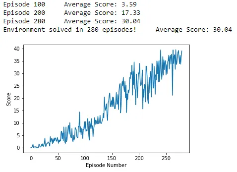
A score of +30 achieved in 280 episodes
CONCLUSION
The results achieved as showcased above during training were achieved after a number of unsuccessful starts with a different set of hyperparameters and neural-net architectures than the ones finally used. To summarize from the experience a simple neural-net architecture with maximum of 2–3 hidden layers for both Actor and Critic works best for this implementation and the key game-changer was introduction of noise decay parameter during training to prefer exploration over exploitation during initial stages of training and then prefer exploitations over exploration during later stages because by then the agent has been made to learn and train enough and it should then be given a chance to implement its learning to select actions for achieving the desired goal besides exploring the environment still but at a relatively lesser proportion than during the initial stages of training. This approach helped in accelerating the training process manifold and way quicker convergence to estimation of network weights of the optimal policy as the agent hence achieved the target goal score just within 300 episodes compared to more than 2000 episodes in previous attempts. Also I used gradient clipping when training the critic network to stabilize the training process of the agent which seems to have helped in achieving the desired result.
Installation Instructions to setup the Project :
1) Setting Up Python Environment :
a) Download and install Anaconda 3 (latest version 5.3) from this link (https://www.anaconda.com/download/)for the specific Operating System and Architecture (64-bit or 32-bit) being used for Python 3.6 + version onwards

b) Create (and activate) a new environment with Python 3.6.:
   Open Anaconda prompt and then execute the below given commands

   Linux or Mac:
   conda create --name drlnd python=3.6
   source activate drlnd

   Windows:
   conda create --name drlnd python=3.6
   activate drlnd

 c) Minimal Installation of OpenAi Gym Environment
    Below are the instructions to do minimal install of gym :

    git clone https://github.com/openai/gym.git
    cd gym
    pip install -e .

    A minimal install of the packaged version can be done directly from PyPI: pip install gym

 d) Clone the repository (https://github.com/udacity/deep-reinforcement-learning.git) and navigate to the python/ folder.
Then, install several dependencies by executing the below commands in Anaconda Prompt Shell :
git clone https://github.com/udacity/deep-reinforcement-learning.git
cd deep-reinforcement-learning/python
pip install . (or pip install [all] )

 e) Create an Ipython Kernel for the drlnd environment :
python -m ipykernel install --user --name drlnd --display-name "drlnd"

 f) Before running code in a notebook, change the kernel to match the drlnd environment by using the drop-down Kernel menu.
2) Install Unity ML-Agents associated libraries/modules:
Clone the GitHub Repository (https://github.com/Unity-Technologies/ml-agents.git)
and install the required libraries by running the below mentioned commands in the Anaconda Prompt

git clone https://github.com/Unity-Technologies/ml-agents.git
cd ml-agents/ml-agents (navigate inside ml-agents subfolder)
pip install . or (pip install [all]) (install the modules required)
3) Download the Unity Environment :
a) For this project, Unity is not necessary to be installed because readymade built environment has already been provided, and can be downloaded from one of the links below as per the operating system being used:

Single-Agent Reacher Environment :
   Linux: https://s3-us-west-1.amazonaws.com/udacity-drlnd/P2/Reacher/one_agent/Reacher_Linux.zip
   Mac OSX: https://s3-us-west-1.amazonaws.com/udacity-drlnd/P2/Reacher/one_agent/Reacher.app.zip
   Windows (32-bit): https://s3-us-west-1.amazonaws.com/udacity-drlnd/P2/Reacher/one_agent/Reacher_Windows_x86.zip
   Windows (64-bit): https://s3-us-west-1.amazonaws.com/udacity-drlnd/P2/Reacher/one_agent/Reacher_Windows_x86_64.zipPlace the downloaded file in the p2_continuous-control/ as well as python/ folder in the DRLND GitHub repository, and unzip (or decompress) the file.

c) (For AWS) If the agent is to be trained on AWS (and a virtual screen is not enabled), then please use this link
(https://s3-us-west-1.amazonaws.com/udacity-drlnd/P2/Reacher/one_agent/Reacher_Linux_NoVis.zip) for Single-Agent
Reacher Environment to obtain the "headless" version of the environment. Watching the agent during training is not possible without enabling a virtual screen.(To watch the agent , follow the instructions to enable a virtual screen (https://github.com/Unity-Technologies/ml-agents/blob/master/docs/Training-on-Amazon-Web-Service.md)and then download the environment for the Linux operating  system above.)
Details of running the Code to Train the Agent / Test the Already Trained Agent :
- First of all clone this repository (https://github.com/PranayKr/Deep_Reinforcement_Learning_Projects.git) on local system.
- Also clone the repository (https://github.com/udacity/deep-reinforcement-learning.git) mentioned previously on local system.
- Now place all the Source code files and pretrained model weights present in this cloned GitHub Repo inside the python/ folder of the Deep-RL cloned repository folder.
- Next place the folder containing the downloaded unity environment file for Windows (64-bit) OS inside the python/ folder of the Deep-RL cloned repository folder.
- Open Anaconda prompt shell window and navigate inside the python/ folder in the Deep-RL cloned repository folder.
- Run the command “jupyter notebook” from the Anaconda prompt shell window to open the jupyter notebook web-app tool in the browser from where any of the provided training and testing source codes present in notebooks(.ipynb files) can be opened.
- Before running/executing code in a notebook, change the kernel (IPython Kernel created for drlnd environment) to match the drlnd environment by using the drop-down Kernel menu.
- The source code present in the provided training and testing notebooks(.ipynb files) can also be collated in respective new python files(.py files) and then executed directly from the Anaconda prompt shell window using the command “python <filename.py>”.
NOTE:
- All the cells can executed at once by choosing the option (Restart and Run All) in the Kernel Tab.
- Please change the name of the (*.pth) file where the model weights are getting saved during training to avoid overwriting of already existing pre-trained model weights existing currently with the same filename.
Deep Deterministic Policy Gradient (DDPG) Algorithm Training / Testing Details (Files Used) :
For Training : Open the below mentioned Jupyter Notebook and execute all the cells
Continuous_Control-Reacher_SingleAgent_DDPG_WorkingSoln.ipynb

Neural Net Model Architecture file Used : ModelTest.py
The Unity Agent file used : Test2_Agent.py

For Testing : open the Jupyter Notebook file "DDPGAgent_Test.ipynb" and run the code to test the results obtained using Pre-trained model weights for Actor Neural-Net Model and Critic Neural-Net Model

Pretrained Model Weights provided : 1) checkpoint_actor.pth
                                    2) checkpoint_critic.pth
REFERENCES :
- CONTINUOUS CONTROL WITH DEEP REINFORCEMENT LEARNING (https://arxiv.org/pdf/1509.02971.pdf)
- Benchmarking Deep Reinforcement Learning for Continuous Control (https://arxiv.org/pdf/1604.06778.pdf)
- An implementation of DDPG with OpenAI Gym’s Pendulum environment (https://github.com/udacity/deep-reinforcement-learning/tree/master/ddpg-pendulum)
- An implementation of DDPG with OpenAI Gym’s BipedalWalker environment (https://github.com/udacity/deep-reinforcement-learning/tree/master/ddpg-bipedal)
NOTE :
- This article is also published in LinkedIn ( https://www.linkedin.com/pulse/robotic-arm-gripper-trained-hold-object-using-deep-learning-kumar )
- If you wish to connect drop me a message over LinkedIn ( https://www.linkedin.com/in/pranay-kumar-02b35524/ ) or email at pranay.scorpio9@gmail.com
