Linear Regression Part 1

Linear Regression is the simplest type of Supervised learning.

The goal of Regression is to explore the relation between the input Feature with that of the target Value and give us a continuous Valued output for the given unknown data.

This is a General data Flow diagram of a linear regression model

In linear regression the we explore the relation between input and target with a linear equation. For a simple linear regression model with only one feature the Equation becomes:

Y=W1*X+b

• Y=Predicted value/Target Value
• X=Input
• W1=Gradient/slope/Weight
• b=Bias

The equation is same as that of a straight line (Y=MX+c)

What the question arises what is this W1 and b?

— —> For now lets say they are the parameters to adjust the straight line to get the best fit. By adjusting the W1 and b we get the algorithm to get the most optimized results.

Multiple Regression:

Now we have a set of input features X={x1,x2,x3,….,xn} and weights associated with it W={w1,w2,w3,….wn}. Thus the equation becomes:

Y=(x1*w1+x2*w2+x3*w3+....+xn*wn)

or

Multiple regression Equation

With bias consideration

Y=(x1*w1+x2*w2+x3*w3+….+xn*wn)+b

or

Multiple regression Equation with bias

Now lets come back to the weights :

How do we determine the weights and bias?

=> The weights are are measured by MSE (Mean Squared Error) and adjusting them to get a best possible Linear line.

MSE =average of ((predicted value — actual value of i th value of y)²)

Image1 from(https://cdn-images-1.medium.com/max/1200/0*FjKhbw6Va8O8bCkF.png)

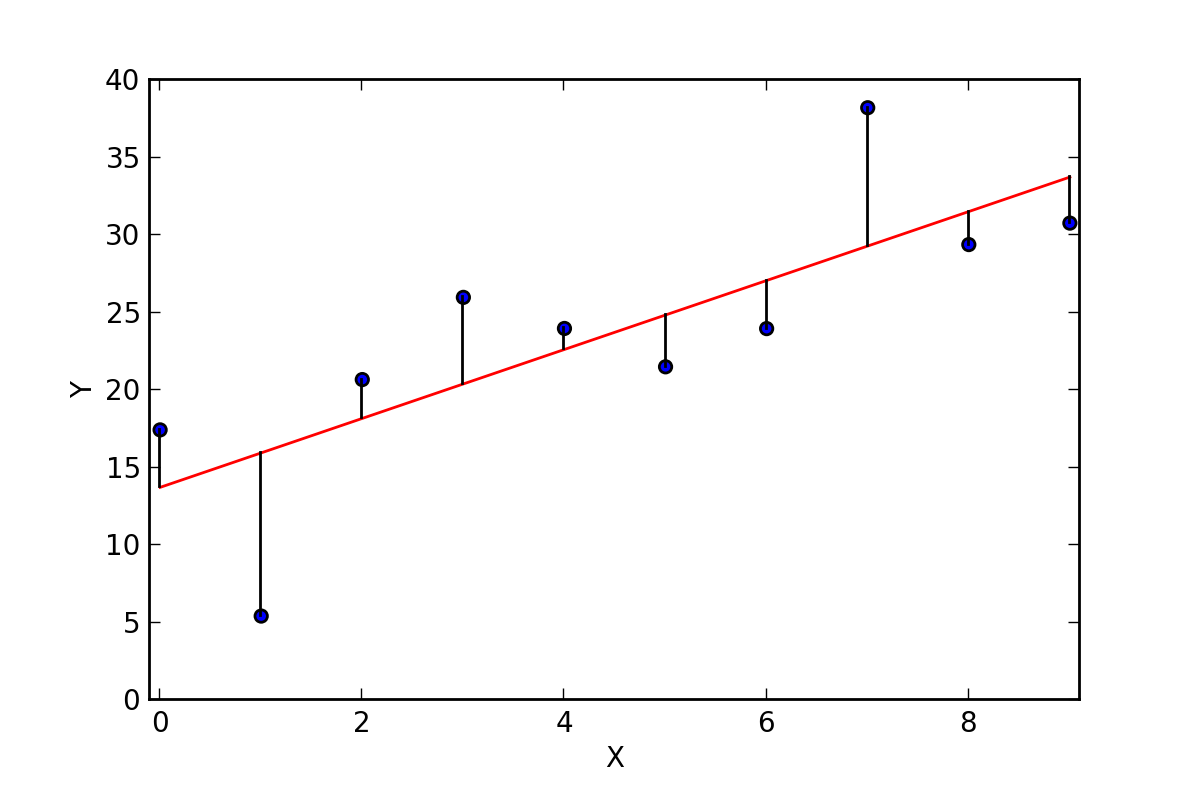
Let us understand the concept from image1 — the ‘red line’ is our linear regression line or our predicted value(y’). And the ‘blue’ points are our given data or actual value. The average of square of distance from the blue points(actual value) to the red line(predicted value) must be minimum to get the best fit regression line.

Thus can be represented as

MSE where y’ is predicted value yi is actual value

To gain optimal result we need to minimize MSE

So to minimize this error or MSE we use gradient descent to find the weights after MSE or error rate calculation. Gradient Descent can be Equated as :

Gradient Descent

Now after we get the Gradient descent we need to update the weight every time until we get the best fitted value

new Weight=old Weight+(Learning Rate *Gradient Descent)

new Weight=old Weight+(Learning Rate *Gradient Descent)

alpha or learning rate is fixed value ranging between 0–1, at this moment we don’t need to know much of it. In the next article I will explain how multiple regression works.

Now lets see the coding part:

What we need

• python 3.6+ Download Python
• pandas library (pip3 install pandas)
• matplotlib library (pip3 install matplotlib)
• scikitlearn library (pip3 install sklearn)
• CSV file : https://github.com/neelindresh/NeelBlog/blob/master/HousePrice.csv

Code: for simple regression
import pandas
#load csv file
df=pandas.read_csv('./DataSet/HousePrice.csv')
df=df[['Price (Older)', 'Price (New)']]
#Define feature list (X) target(Y)
X=df[['Price (Older)']]
Y=df[['Price (New)']]
#load predefined linearRegression model
from sklearn.model_selection import train_test_split
from sklearn.linear_model import LinearRegression
xTrain,xTest,yTrain,yTest=train_test_split(X,Y)
Lreg=LinearRegression().fit(xTrain,yTrain)
#   formula=(W1*x+b)
print('Coef(W1):',Lreg.coef_)
print('Intercept(W0/b):',Lreg.intercept_)
W1=Lreg.coef_
b=Lreg.intercept_
#ploting the same
import matplotlib.pyplot as plt
plt.scatter(X,Y)
plt.plot(X,W1*X+b,'r-')
plt.show()
#You can predict a value using
#print(Lreg.predict(someValue))

the full code and csv file is available at : Download from github

Output

Output graph

Description:

The CSV file had a number of columns . But I used only two of them to show how simple regression works. ‘Price (Older)’ VS ‘Price (New)’ where ‘older’ is the x coordinate and ‘new’ is the y coordinate.

Loading the CSV file

df=pandas.read_csv(‘./DataSet/HousePrice.csv’)

Slicing the ‘Price (Older)’ ‘Price (New)’ columns from the data frame:

df=df[[‘Price (Older)’, ‘Price (New)’]]

Define feature list (X) target(Y)

X=df[[‘Price (Older)’]]
Y=df[[‘Price (New)’]]

TrainTestSplit divides the data set in 75% training 25% testing data

xTrain,xTest,yTrain,yTest=train_test_split(X,Y)

LinearRegression().fit(X,Y)-> puts the x values and y values in the given function respectively

Lreg=LinearRegression().fit(xTrain,yTrain)

The W1 and b (final weight and final bias) which gives the best fit

W1=Lreg.coef_
b=Lreg.intercept_

Plotting using matPlotLib

#ploting the same
import matplotlib.pyplot as plt
plt.scatter(X,Y)
plt.plot(X,W1*X+b,'r-')
plt.show()

You can predict the a value using:

print(Lreg.predict(someValue))

Follow me on youtube:

Neel Bhattacharyya

Follow my blog:

Data Science for Everyone