Using Multilayer Perceptron in Iris Flower DataSet

Published in

Computing Science

5 min readAug 28, 2019

Introduction

The Iris Flower Dataset, also called Fisher’s Iris, is a dataset introduced by Ronald Fisher, a British statistician, and biologist, with several contributions to science. Ronald Fisher has well known worldwide for his paper The use of multiple measurements in taxonomic problems as an example of linear discriminant analysis. It was in this paper that Ronald Fisher introduced the Iris flower dataset.

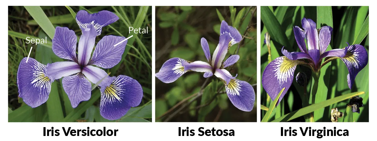
The iris database consists of 50 samples distributed among three different species of iris. Each of these samples has specific characteristics, which allows them to be classified into three categories: Iris Setosa, Iris Virginica, and Iris versicolor. In this tutorial, we will use multilayer perceptron to separate and classify the iris samples.

Details about the iris data set

The data set consists of 50 samples from each of three species of Iris (Iris setosa, Iris virginica, and Iris versicolor).
Four features were measured from each sample, the length and the width of the sepals and petals, in centimeters.
Based on the combination of these four features, Fisher developed a linear discriminant model to distinguish the species from each other.

Using MLP without libraries

In this example, we will implement a multilayer perceptron without any Python libraries. However, to help us format and manipulate the iris data set, we will use numpy, matplotlib, seaborn, and scikit-learn libraries.

A prior analysis of the problem

Before, It is necessary to define some things about the problem. First, We have 4-inputs related to each y output. Our number of instances is equal to 150 samples (50 in each of three classes to classification).

The x inputs are arranged as follows (computational notation):

For the variable xat position x[0], we have the attribute: sepal width;
For the variable xat position x[1], we have the attribute: sepal length;
For the variable xat position x[2], we have the attribute: petal width;
For the variable xat position x[3], we have the attribute: petal length;

The y outputs are arranged as follows (computational notation):

For categorization, the condition is if y = 0 then: Iris Setosa;
For categorization, the condition isif y = 1 then: Iris Versicolor;
For categorization, the condition isif y = 2 then: Iris Virginica;

Plotting iris data set with matplotlib

Separating samples in the iris flower data set

To perform this tutorial, we have divided 80% of the training samples and 20% for the test samples.

Artificial Neural Network (ANN)

Artificial neural networks (ANNs) or connectionist systems are computing systems inspired by the biological neural networks that constitute animal brains. The neural networks deliver new functionality to the computer, the ability to learn and progressively improve performance with each further interaction.

Briefly, we can describe artificial neural networks as computational techniques or mathematical models that simulate the functioning of biological neurons. In this context, each artificial neuron acts as processing units in a neural network.

Multilayer Perceptron

The Multilayer Perceptron Networks are characterized by the presence of many intermediate layers (hidden) in your structure, located between the input layer and the output layer. With this, such networks have the advantage of being able to classify more than two different classes, and It also solves non-linearly separable problems.

The Multilayer networks can classify nonlinearly separable problems, one of the limitations of single-layer Perceptron. For this reason, the Multilayer Perceptron is a candidate to serve on the iris flower data set classification problem.

How does Multilayer Perceptron really work?

We can summarize the operation of the perceptron as follows it:

Step 1: Initialize the weights and bias with small-randomized values;

Step 2: Propagate all values in the input layer until the output layer (Forward Propagation);

Step 3: Update weight and bias in the inner layers(Backpropagation);

Step 4: Do it until that the stop criterion is satisfied!

Forward propagation

In order to proceed, we need to improve the notation we have been using. That for, for each layer 1≥ l≥ L≥, the activations and outputs are calculated as: